

Carry this undertaking to life
One of many points which plague deep studying fashions is the truth that they usually have no idea what they have no idea. That being the case fashions may want an added layer of safety in opposition to knowledge courses which they haven’t been uncovered to throughout coaching. On this article, we’ll take a look at one in every of such strategies intimately.
#  article dependencies
import torch
import torch.nn as nn
import torch.nn.practical as F
import torchvision
import torchvision.transforms as transforms
import torchvision.datasets as Datasets
from torch.utils.knowledge import Dataset, DataLoader
import numpy as np
import matplotlib.pyplot as plt
import cv2
from tqdm.pocket book import tqdm
from tqdm import tqdm as tqdm_regular
import seaborn as sns
from torchvision.utils import make_grid
import random
if torch.cuda.is_available():
machine = torch.machine('cuda:0')
print('Operating on the GPU')
else:
machine = torch.machine('cpu')
print('Operating on the CPU')Uncertainty in Deep Studying
Like I had talked about within the overview, deep studying fashions usually do not know what they do not know. As an illustration think about a mannequin educated to categorise handwritten digits contained within the MNIST dataset, if a picture of a desk is provided to stated mannequin it’s going to classify this desk as both one of many ten handwritten picture courses with out hesitation. In precise truth, what the mannequin does is to return a vector containing confidence scores for every class after which now we have some logic to select the best rating and classify the picture accordingly.
The mannequin has no inherent capability to interject and infer that it has not been uncovered to a sure form of picture throughout coaching and simply goes forward to deal with it as regular. This lack of discernment on the mannequin’s half is time period uncertainty. When the mannequin acts on out-of-sample knowledge (knowledge from a category not current within the coaching set) and treats it as regular that is referred to as aleatoric/knowledge uncertainty. Nevertheless when a mannequin acts on in-sample knowledge however one which is an edge case (appears to be like markedly totally different from these current within the coaching set) and treats it as regular that is referred to as epistemic/mannequin uncertainty. There exists methods of measuring these uncertainties, nevertheless, this text is concentrated on the right way to cease a possible case of aleatoric uncertainty earlier than it occurs.
Handing Aleatoric Uncertainty
Dealing with aleatoric uncertainty on this occasion refers to a technique of including some redundancy to our mannequin such that it is aware of when out-of-sample knowledge is being feed to it. This redundancy will probably be within the type of one other mannequin which has properties making it appropriate for detecting out-of-sample knowledge cases. This course of could be referred to as anomaly detection, and an apparent candidate for this can be a convolutional autoencoder.
Why Convolutional Autoencoders?
As everyone knows, convolutional autoencoders are deep studying neural networks who’s sole function is encoding and decoding of enter pictures with the goal of reconstructing them as they have been. Similar to another supervised studying process, convolution autoencoders are solely appropriate for creating reconstructions (even when they aren’t excellent) of pictures in courses current within the coaching set. If a picture of a category outdoors the coaching set is handed by way of a convolutional autoencoder, it is reconstruction will probably be fairly unsatisfactory.
Herein lies that property that make convolutional autoencoders appropriate for the duty of anomaly detection. When a reconstruction is produced, we are able to measure the reconstruction loss between the unique picture and the reconstruction then evaluate this loss with a predefined threshold in a bid to find out if the picture is out-of-sample or not.
Implementing an Anomaly Detector
Think about an hypothetical situation the place one intends to coach a binary classification mannequin able to classifying cat and canine pictures. On this case, so as to function an anomaly detector, a convolutional autoencoder must be educated to reconstruct solely pictures of cats and canine. For the sake of this text, these pictures will probably be gotten from the CIFAR-10 dataset.
def extract_images(dataset):
  """
  This perform extracts pictures of cats (index 3)
  and canine (index 5) from the CIFAR-10 dataset.
  """
  cats = []
  canine = []

  for idx in tqdm_regular(vary(len(dataset))):
    if dataset.targets[idx]==3:
      cats.append((dataset.knowledge[idx], 0))
    elif dataset.targets[idx]==5:
      canine.append((dataset.knowledge[idx], 1))
    else:
      go
  return cats, canine


#  loading coaching knowledge
training_set = Datasets.CIFAR10(root="./", obtain=True,
                              remodel=transforms.ToTensor())

#  loading validation knowledge
validation_set = Datasets.CIFAR10(root="./", obtain=True, prepare=False,
                                remodel=transforms.ToTensor())


#  extracting coaching pictures
cat_train, dog_train = extract_images(training_set)
training_data = cat_train + dog_train
random.shuffle(training_data)

#  extracting validation pictures
cat_val, dog_val = extract_images(validation_set)
validation_data = cat_val + dog_val
random.shuffle(training_data)


#  eradicating labels
training_images = [x[0] for x in training_data]
validation_images = [x[0] for x in validation_data]
test_images = [x[0] for x in cat_val[:5]] + [x[0] for x in dog_val[:5]]
Having extracted the photographs and allotted them to their proper objects, it’s now time to create a PyTorch dataset which is able to enable them for use for coaching a PyTorch mannequin.
#  defining dataset class
class CustomCIFAR10(Dataset):
  def __init__(self, knowledge, transforms=None):
    self.knowledge = knowledge
    self.transforms = transforms

  def __len__(self):
    return len(self.knowledge)

  def __getitem__(self, idx):
    picture = self.knowledge[idx]

    if self.transforms!=None:
      picture = self.transforms(picture)
    return picture


#  creating pytorch datasets
training_data = CustomCIFAR10(training_images, transforms=transforms.Compose([transforms.ToTensor(),
                                                                              transforms.Normalize((0.5, 0.5, 0.5), (0.5, 0.5, 0.5))]))
validation_data = CustomCIFAR10(validation_images, transforms=transforms.Compose([transforms.ToTensor(),
                                                                                  transforms.Normalize((0.5, 0.5, 0.5), (0.5, 0.5, 0.5))]))
test_data = CustomCIFAR10(test_images, transforms=transforms.Compose([transforms.ToTensor(),
                                                                                  transforms.Normalize((0.5, 0.5, 0.5), (0.5, 0.5, 0.5))]))
Convolutional Autoencoder Structure
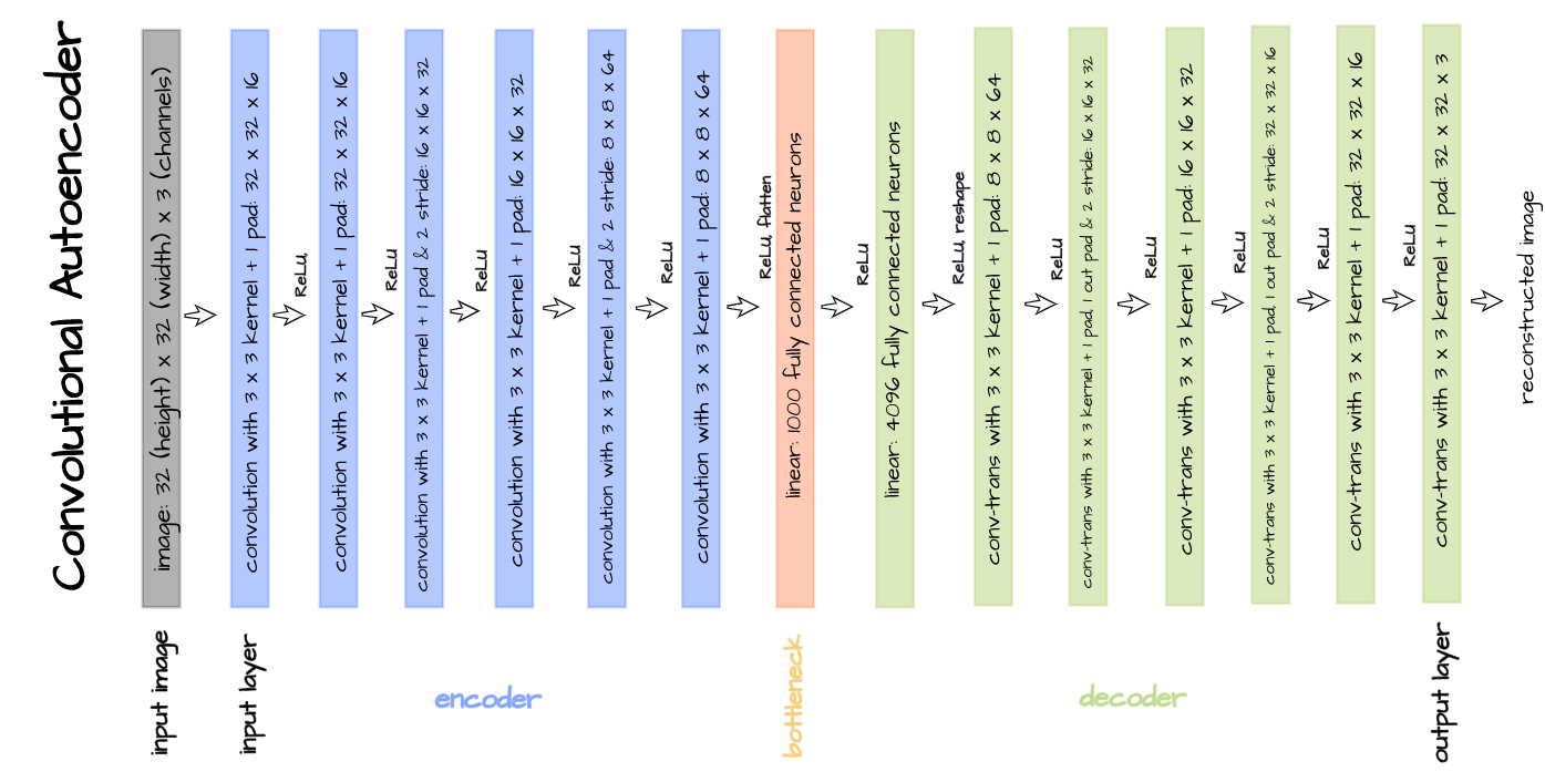
The above illustrated convolutional autoencoder structure will probably be applied for the aims of this text. Implementation is completed by defining the encoder and decoder as distinct courses with the bottleneck connected as the ultimate layer within the encoder. Thereafter, each courses are mixed as one in an autoencoder class.
#  defining encoder
class Encoder(nn.Module):
  def __init__(self, in_channels=3, out_channels=16, latent_dim=1000, act_fn=nn.ReLU()):
    tremendous().__init__()

    self.web = nn.Sequential(
        nn.Conv2d(in_channels, out_channels, 3, padding=1), # (32, 32)
        act_fn,
        nn.Conv2d(out_channels, out_channels, 3, padding=1),
        act_fn,
        nn.Conv2d(out_channels, 2*out_channels, 3, padding=1, stride=2), # (16, 16)
        act_fn,
        nn.Conv2d(2*out_channels, 2*out_channels, 3, padding=1),
        act_fn,
        nn.Conv2d(2*out_channels, 4*out_channels, 3, padding=1, stride=2), # (8, 8)
        act_fn,
        nn.Conv2d(4*out_channels, 4*out_channels, 3, padding=1),
        act_fn,
        nn.Flatten(),
        nn.Linear(4*out_channels*8*8, latent_dim),
        act_fn
    )

  def ahead(self, x):
    x = x.view(-1, 3, 32, 32)
    output = self.web(x)
    return output


#  defining decoder
class Decoder(nn.Module):
  def __init__(self, in_channels=3, out_channels=16, latent_dim=1000, act_fn=nn.ReLU()):
    tremendous().__init__()

    self.out_channels = out_channels

    self.linear = nn.Sequential(
        nn.Linear(latent_dim, 4*out_channels*8*8),
        act_fn
    )

    self.conv = nn.Sequential(
        nn.ConvTranspose2d(4*out_channels, 4*out_channels, 3, padding=1), # (8, 8)
        act_fn,
        nn.ConvTranspose2d(4*out_channels, 2*out_channels, 3, padding=1,
                           stride=2, output_padding=1), # (16, 16)
        act_fn,
        nn.ConvTranspose2d(2*out_channels, 2*out_channels, 3, padding=1),
        act_fn,
        nn.ConvTranspose2d(2*out_channels, out_channels, 3, padding=1,
                           stride=2, output_padding=1), # (32, 32)
        act_fn,
        nn.ConvTranspose2d(out_channels, out_channels, 3, padding=1),
        act_fn,
        nn.ConvTranspose2d(out_channels, in_channels, 3, padding=1)
    )

  def ahead(self, x):
    output = self.linear(x)
    output = output.view(-1, 4*self.out_channels, 8, 8)
    output = self.conv(output)
    return output


#  defining autoencoder
class Autoencoder(nn.Module):
  def __init__(self, encoder, decoder):
    tremendous().__init__()
    self.encoder = encoder
    self.encoder.to(machine)

    self.decoder = decoder
    self.decoder.to(machine)

  def ahead(self, x):
    encoded = self.encoder(x)
    decoded = self.decoder(encoded)
    return decoded
Convolutional Neural Community Class
The category beneath is outlined to mix coaching, validation in addition to different functionalities of our convolutional autoencoder.
class ConvolutionalAutoencoder():
  def __init__(self, autoencoder):
    self.community = autoencoder
    self.optimizer = torch.optim.Adam(self.community.parameters(), lr=1e-3)

  def prepare(self, loss_function, epochs, batch_size,
            training_set, validation_set, test_set):

    #  creating log
    log_dict = {
        'training_loss_per_batch': [],
        'validation_loss_per_batch': [],
        'visualizations': []
    }

    #  defining weight initialization perform
    def init_weights(module):
      if isinstance(module, nn.Conv2d):
        torch.nn.init.xavier_uniform_(module.weight)
        module.bias.knowledge.fill_(0.01)
      elif isinstance(module, nn.Linear):
        torch.nn.init.xavier_uniform_(module.weight)
        module.bias.knowledge.fill_(0.01)

    #  initializing community weights
    self.community.apply(init_weights)

    #  creating dataloaders
    train_loader = DataLoader(training_set, batch_size)
    val_loader = DataLoader(validation_set, batch_size)
    test_loader = DataLoader(test_set, 10)

    #  setting convnet to coaching mode
    self.community.prepare()
    self.community.to(machine)

    for epoch in vary(epochs):
      print(f'Epoch {epoch+1}/{epochs}')
      train_losses = []

      #------------
      #  TRAINING
      #------------
      print('coaching...')
      for pictures in tqdm(train_loader):
        #  zeroing gradients
        self.optimizer.zero_grad()
        #  sending pictures to machine
        pictures = pictures.to(machine)
        #  reconstructing pictures
        output = self.community(pictures)
        #  computing loss
        loss = loss_function(output, pictures.view(-1, 3, 32, 32))
        #  calculating gradients
        loss.backward()
        #  optimizing weights
        self.optimizer.step()

        #--------------
        # LOGGING
        #--------------
        log_dict['training_loss_per_batch'].append(loss.merchandise())

      #--------------
      # VALIDATION
      #--------------
      print('validating...')
      for val_images in tqdm(val_loader):
        with torch.no_grad():
          #  sending validation pictures to machine
          val_images = val_images.to(machine)
          #  reconstructing pictures
          output = self.community(val_images)
          #  computing validation loss
          val_loss = loss_function(output, val_images.view(-1, 3, 32, 32))

        #--------------
        # LOGGING
        #--------------
        log_dict['validation_loss_per_batch'].append(val_loss.merchandise())


      #--------------
      # VISUALISATION
      #--------------
      print(f'training_loss: {spherical(loss.merchandise(), 4)} validation_loss: {spherical(val_loss.merchandise(), 4)}')

      for test_images in test_loader:
        #  sending check pictures to machine
        test_images = test_images.to(machine)
        with torch.no_grad():
          #  reconstructing check pictures
          reconstructed_imgs = self.community(test_images)
        #  sending reconstructed and pictures to cpu to permit for visualization
        reconstructed_imgs = reconstructed_imgs.cpu()
        test_images = test_images.cpu()

        #  visualisation
        imgs = torch.stack([test_images.view(-1, 3, 32, 32), reconstructed_imgs],
                          dim=1).flatten(0,1)
        grid = make_grid(imgs, nrow=10, normalize=True, padding=1)
        grid = grid.permute(1, 2, 0)
        plt.determine(dpi=170)
        plt.title('Authentic/Reconstructed')
        plt.imshow(grid)
        log_dict['visualizations'].append(grid)
        plt.axis('off')
        plt.present()

    return log_dict

  def autoencode(self, x):
    return self.community(x)

  def encode(self, x):
    encoder = self.community.encoder
    return encoder(x)

  def decode(self, x):
    decoder = self.community.decoder
    return decoder(x)
Coaching and Validation
Carry this undertaking to life
With every little thing in the suitable order, it’s now time to coach our convolutional autoencoder. The autoencoder is educated with parameters as outlined within the code cell beneath.
# coaching mannequin
mannequin = ConvolutionalAutoencoder(Autoencoder(Encoder(), Decoder()))
log_dict = mannequin.prepare(nn.MSELoss(), epochs=30, batch_size=64,
training_set=training_data, validation_set=validation_data,
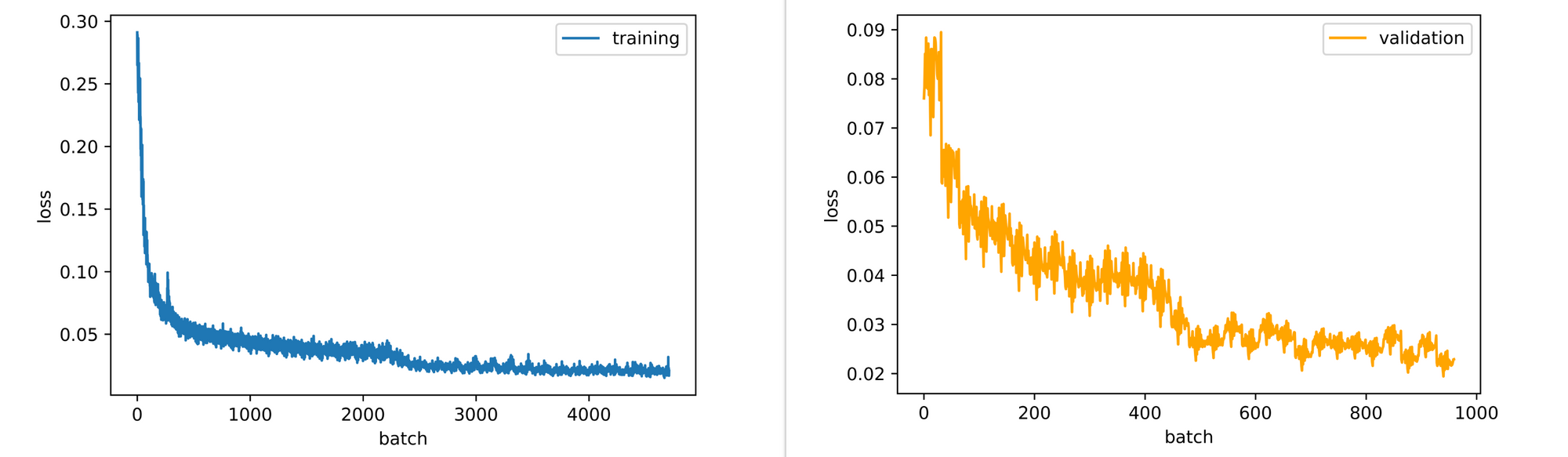
test_set=test_data)From the visualizations and losses returned on the finish of every epoch, it may be seen that the autoencoder regularly learns the right way to reconstruct pictures even when they’re nonetheless blurry on the finish of the thirtieth epoch (be happy to coach for longer).
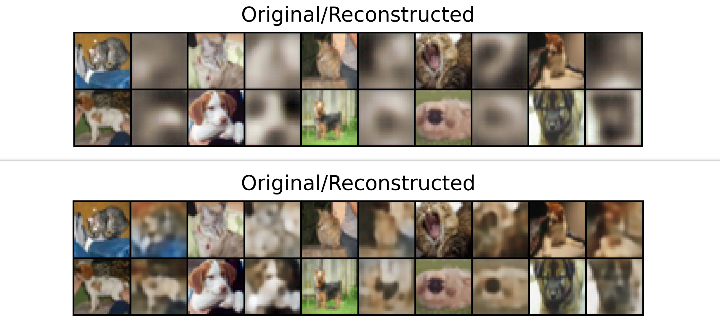
Additionally, the coaching and validation loss plots are nonetheless barely down-trending so the mannequin may profit from some further epochs of coaching.
Computing Reconstruction Loss
The perform beneath accepts a picture as parameter then proceeds to go stated picture by way of the already educated convolutional autoencoder so as to derive a reconstruction of the picture. Thereafter, imply squared error is used to measure reconstruction loss between the uploaded picture and it is reconstruction. Utilizing this perform we will probably be deriving reconstruction loss for some pictures in a bid to find out a attainable baseline for out-of-sample knowledge (anomalies).
def reconstruction_loss(picture, mannequin, visualize=True):
  """
  This perform calculates the reconstruction lack of an
  picture for anomaly detection
  """
  #  studying picture
  picture = cv2.imread(picture)
  picture = cv2.cvtColor(picture, cv2.COLOR_BGR2RGB)
  picture = cv2.resize(picture, (32, 32))

  #  defining transforms
  remodel =transforms.Compose([transforms.ToTensor(),
                                 transforms.Normalize((0.5, 0.5, 0.5), (0.5, 0.5, 0.5))])
  picture = remodel(picture)
  picture = picture.view(-1, 3, 32, 32)
  picture = picture.to(machine)

  #  passing picture by way of autoencoder
  with torch.no_grad():
    reconstruction = mannequin.autoencode(picture)
    #  computing reconstruction loss
    reconstruction_loss = F.mse_loss(picture, reconstruction)

  print(f'reconstruction_loss: {spherical(reconstruction_loss.merchandise(), 4)}')

  if visualize:
    #  visualization
    grid = make_grid([image.view(3, 32, 32).cpu(), reconstruction.view(3, 32, 32).cpu()], normalize=True, padding=1)
    grid = grid.permute(1,2,0)
    plt.determine(dpi=100)
    plt.title('uploaded/reconstruction')
    plt.axis('off')
    plt.imshow(grid)
  else:
    go

  return spherical(reconstruction_loss.merchandise(), 4)
Cat Picture 1
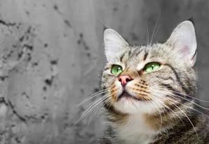
On the subject of the cat picture above, when handed by way of the autoencoder we count on it to be moderately reconstructed so we count on a low reconstruction loss. A reconstruction lack of 0.04 is returned however we’d like extra samples earlier than we are able to outline a baseline near that worth.
#  computing loss
recon_loss = reconstruction_loss('cat_1.jpg', mannequin=mannequin)

# >>> reconstruction_loss: 0.0447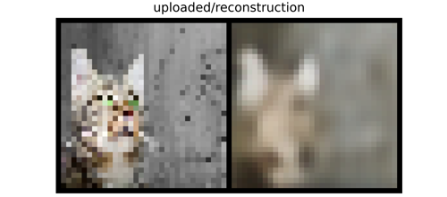
Cat Picture 2

Simply to make certain, let’s attempt one other cat picture to see how properly the autoencoder reconstructs the picture. Upon passing a brand new cat picture by way of the autoencoder, a reconstruction lack of roughly 0.02 is returned, decrease than the primary picture.
#  computing loss
recon_loss = reconstruction_loss('cat_2.jpg', mannequin=mannequin)

# >>> reconstruction_loss: 0.0191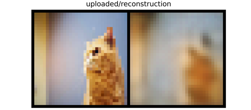
Canine Picture 1
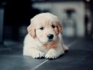
Because the convolutional autoencoder is educated to reconstruct each cat and canine pictures then we’re required to verify it is reconstruction of canine pictures as properly. When the picture above is handed by way of the autoencoder a reconstruction lack of about 0.04 is once more returned, just like the primary cat picture.
#  computing loss
recon_loss = reconstruction_loss('dog_1.jpg', mannequin=mannequin)

# >>> reconstruction_loss: 0.0354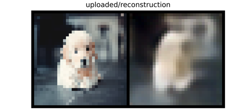
Canine Picture 2
Maintaining with the theme, once more let’s attempt our mannequin on one other canine picture, the one illustrated above. Upon passing this picture by way of the autoencoder, a reconstruction lack of roughly 0.04 is returned, a similar as two of the final 3 pictures.
#  computing loss
recon_loss = reconstruction_loss('dog_2.jpg', mannequin=mannequin)

# >>> reconstruction_loss: 0.0399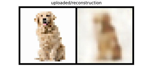
Out-of-Pattern picture 1
Already, we’re getting a way that the autoencoder reconstructs in-sample pictures with a lack of 0.04 so a reconstruction lack of round 0.045 – 0.05 will probably be a good baseline. Nevertheless, earlier than we bounce into conclusions, we’d as properly verify the autoencoder in opposition to out-of-sample pictures. Utilizing the frog picture above we are able to see that the perform outputs a reconstruction lack of 0.07 which is significantly greater than any of the in-sample pictures.
#  computing loss
recon_loss = reconstruction_loss('out_of_sample_1.jpg', mannequin=mannequin)

# >>> reconstruction_loss: 0.0726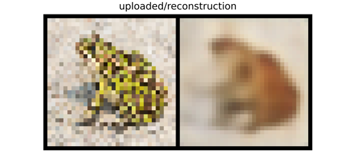
Out-of-Pattern Picture 2

Testing the autoencoder in opposition to one other out of pattern picture yields a reconstruction lack of 0.06. Once more, significantly greater than for in-sample pictures.
#  computing loss
recon_loss = reconstruction_loss('out_of_sample_2.jpg', mannequin=mannequin)

# >>> reconstruction_loss: 0.0581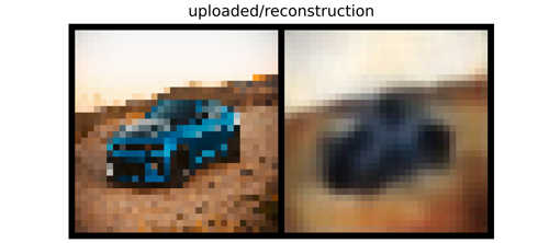
Out-of-Pattern Picture 3
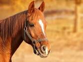
Nevertheless it ought to be famous that anomaly detection with convolutional autoencoders will not be all the time a full proof method. Typical to different fashions in deep studying, autoencoders are additionally inclined to error. Think about the case of the horse picture above, a reconstruction lack of about 0.04 is returned, just like in-sample pictures though that is clearly an out-of-sample picture.
#  computing loss
recon_loss = reconstruction_loss('out_of_sample_3.jpg', mannequin=mannequin)

# >>> reconstruction_loss: 0.037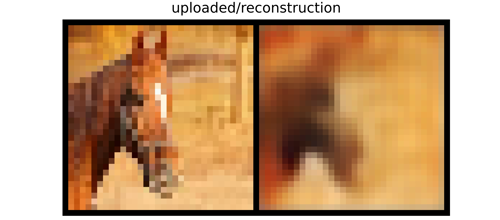
Using the Anomaly Detector
Now that the anomaly detector has been educated and an acceptable baseline established (we’re deciding on 0.045 on this case), we are able to then proceed to make use of it as a display screen for aleatoric uncertainty. To do that, a perform must be written such that any picture which is provided to the mannequin for classification functions first passes by way of the anomaly detector and satisfies the baseline reconstruction loss earlier than being provided unto the mannequin for classification functions.
def aleatoric_screen(picture, mannequin):
  """
  This perform calculates the reconstruction lack of an
  picture and acts as a display screen in opposition to out-of-sample pictures
  """
  #  studying picture
  picture = cv2.imread(picture)
  picture = cv2.cvtColor(picture, cv2.COLOR_BGR2RGB)
  picture = cv2.resize(picture, (32, 32))

  #  defining transforms
  remodel =transforms.Compose([transforms.ToTensor(),
                                 transforms.Normalize((0.5, 0.5, 0.5), (0.5, 0.5, 0.5))])
  picture = remodel(picture)
  picture = picture.view(-1, 3, 32, 32)
  picture = picture.to(machine)

  #  passing picture by way of autoencoder
  with torch.no_grad():
    reconstruction = mannequin.autoencode(picture)
    #  computing reconstruction loss
    reconstruction_loss = F.mse_loss(picture, reconstruction)
    reconstruction_loss = spherical(reconstruction_loss.merchandise(), 3)

  if reconstruction_loss > 0.045:
    print('The mannequin will not be constructed to categorise this type of picture')
  else:
    return picture
On this article, we took a short take a look at uncertainties in deep studying. Thereafter, we took a extra eager take a look at aleatoric uncertainty and the way convolutional autoencoder might help to display screen out-of-sample pictures for classification duties.