Autoencoders and Visual Similarity

Ever questioned how picture search works, or how social media platforms are capable of suggest related pictures to those who you typically like? On this article, we can be looking at one other helpful use of autoencoders, and trying to clarify their utility in laptop imaginative and prescient advice programs.

Setup

We first must import the related packages for the duty at present:

#  article dependencies
import torch
import torch.nn as nn
import torch.nn.practical as F
import torchvision
import torchvision.transforms as transforms
import torchvision.datasets as Datasets
from torch.utils.knowledge import Dataset, DataLoader
import numpy as np
import matplotlib.pyplot as plt
import cv2
from tqdm.pocket book import tqdm
from tqdm import tqdm as tqdm_regular
import seaborn as sns
from torchvision.utils import make_grid
import random
import pandas as pd

We additionally test the machine for a GPU, and allow Torch to run on CUDA if one is obtainable.

#  configuring system
if torch.cuda.is_available():
  system = torch.system('cuda:0')
  print('Working on the GPU')
else:
  system = torch.system('cpu')
  print('Working on the CPU')

Visible Similarity

Within the context of human imaginative and prescient, we people are capable of make comparability between pictures by perceiving their shapes and colours, utilizing this info to entry how related they might be. Nonetheless, relating to laptop imaginative and prescient, to be able to make sense of pictures their options must be extracted first. Thereafter, to be able to examine how related two pictures could also be, their options must be in contrast in some form of method in order to measure similarity in numerical phrases.

The Position of Autoencoders

As we all know, autoencoders are implausible at illustration studying. In reality, they be taught representations effectively sufficient to have the ability to piece collectively pixels and derive the unique picture because it was.

Mainly, an autoencoder’s encoder serves as a characteristic extractor with the extracted options then compressed right into a vector illustration within the bottleneck/code layer. The output of the bottleneck layer on this occasion might be taken as probably the most salient options of a picture which holds an encoding of it is colours and edges. With this encoding of options, one can then proceed to check two pictures in a bid to measure their similarities.

The Cosine Similarity Metric

With a purpose to measure the similarity between the vector representations talked about within the earlier part, we want a metric which is particularly suited to this process. That is the place cosine similarity is available in, a metric which measures the likeness of two vectors by evaluating the angles between them in a vector area.

Not like distance measures like euclidean distance which examine vectors by their magnitudes, cosine similarity is simply involved with climate each vector are pointing in the identical path a property which makes it fairly fascinating for measuring salient similarities.

Using Autoencoders for Visible Similarity

On this part, we’ll prepare an autoencoder then proceed to write down a perform for visible similarity utilizing the autoencoder’s encoder as characteristic extractor and cosine similarity as a metric to evaluate similarity.

Dataset

Typical to articles on this autoencoder collection, we can be utilizing the CIFAR-10 dataset. This dataset incorporates 32 x 32 pixel pictures of objects reminiscent of frogs, horses, automobiles and so forth. The dataset might be loaded utilizing the code cell beneath.

#  loading coaching knowledge
training_set = Datasets.CIFAR10(root="./", obtain=True,
                                rework=transforms.ToTensor())

#  loading validation knowledge
validation_set = Datasets.CIFAR10(root="./", obtain=True, prepare=False,
                                  rework=transforms.ToTensor())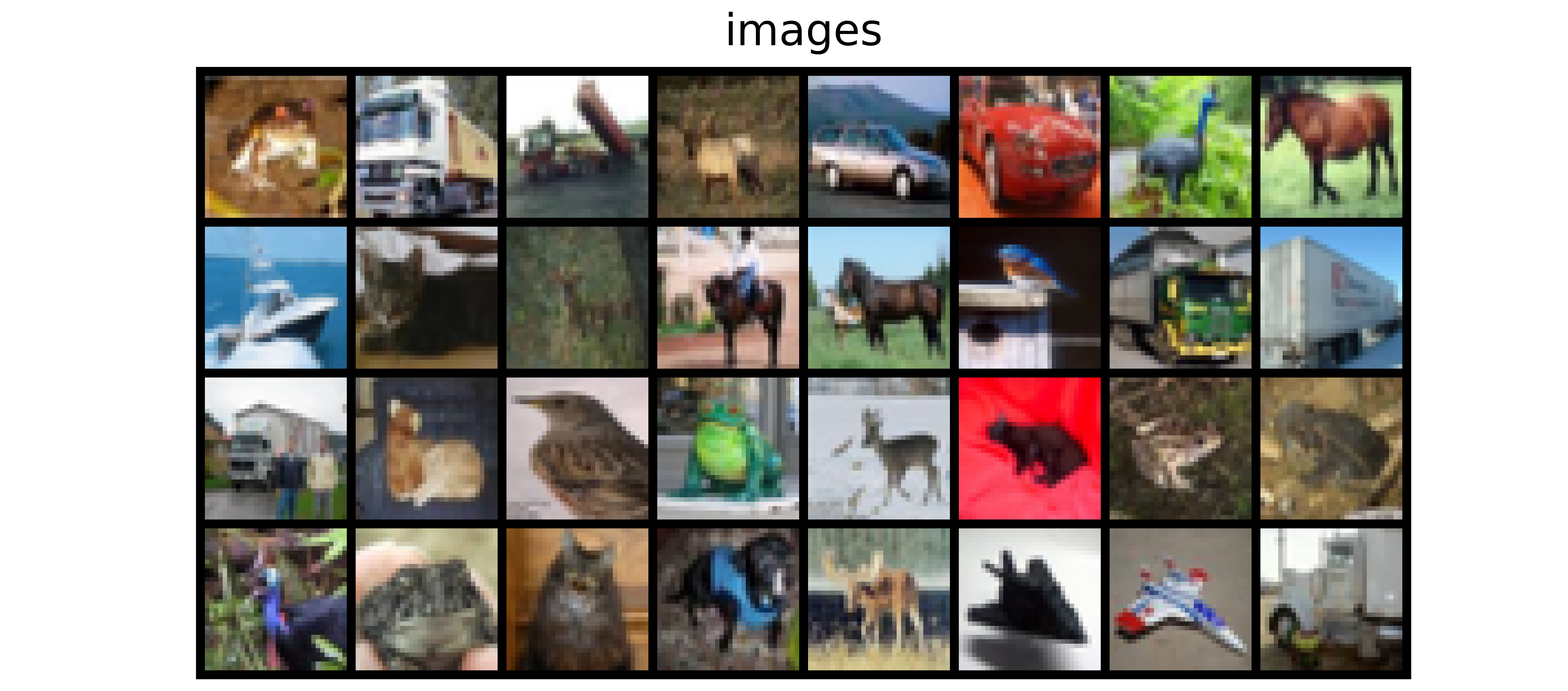

Since we’re coaching an autoencoder which is principally unsupervised, we don’t must class labels which means we are able to simply extract the photographs themselves. For visualization sake, we’ll extract pictures from every class in order to see how effectively the autoencoder does in reconstructing pictures in all courses.

def extract_each_class(dataset):
  """
  This perform searches for and returns
  one picture per class
  """
  pictures = []
  ITERATE = True
  i = 0
  j = 0

  whereas ITERATE:
    for label in tqdm_regular(dataset.targets):
      if label==j:
        pictures.append(dataset.knowledge[i])
        print(f'class {j} discovered')
        i+=1
        j+=1
        if j==10:
          ITERATE = False
      else:
        i+=1

  return pictures
  
  
#  extracting coaching pictures
training_images = [x for x in training_set.data]

#  extracting validation pictures
validation_images = [x for x in validation_set.data]

#  extracting validation pictures
test_images = extract_each_class(validation_set)

Subsequent, we have to outline a PyTorch dataset class in order to have the ability to use our dataset in coaching a PyTorch mannequin. That is carried out within the following code cell.

#  defining dataset class
class CustomCIFAR10(Dataset):
  def __init__(self, knowledge, transforms=None):
    self.knowledge = knowledge
    self.transforms = transforms

  def __len__(self):
    return len(self.knowledge)

  def __getitem__(self, idx):
    picture = self.knowledge[idx]

    if self.transforms!=None:
      picture = self.transforms(picture)
    return picture
    
    
#  creating pytorch datasets
training_data = CustomCIFAR10(training_images, transforms=transforms.Compose([transforms.ToTensor(),
                                                                              transforms.Normalize((0.5, 0.5, 0.5), (0.5, 0.5, 0.5))]))
validation_data = CustomCIFAR10(validation_images, transforms=transforms.Compose([transforms.ToTensor(),
                                                                                  transforms.Normalize((0.5, 0.5, 0.5), (0.5, 0.5, 0.5))]))
test_data = CustomCIFAR10(test_images, transforms=transforms.Compose([transforms.ToTensor(),
                                                                                  transforms.Normalize((0.5, 0.5, 0.5), (0.5, 0.5, 0.5))]))

Autoencoder Structure

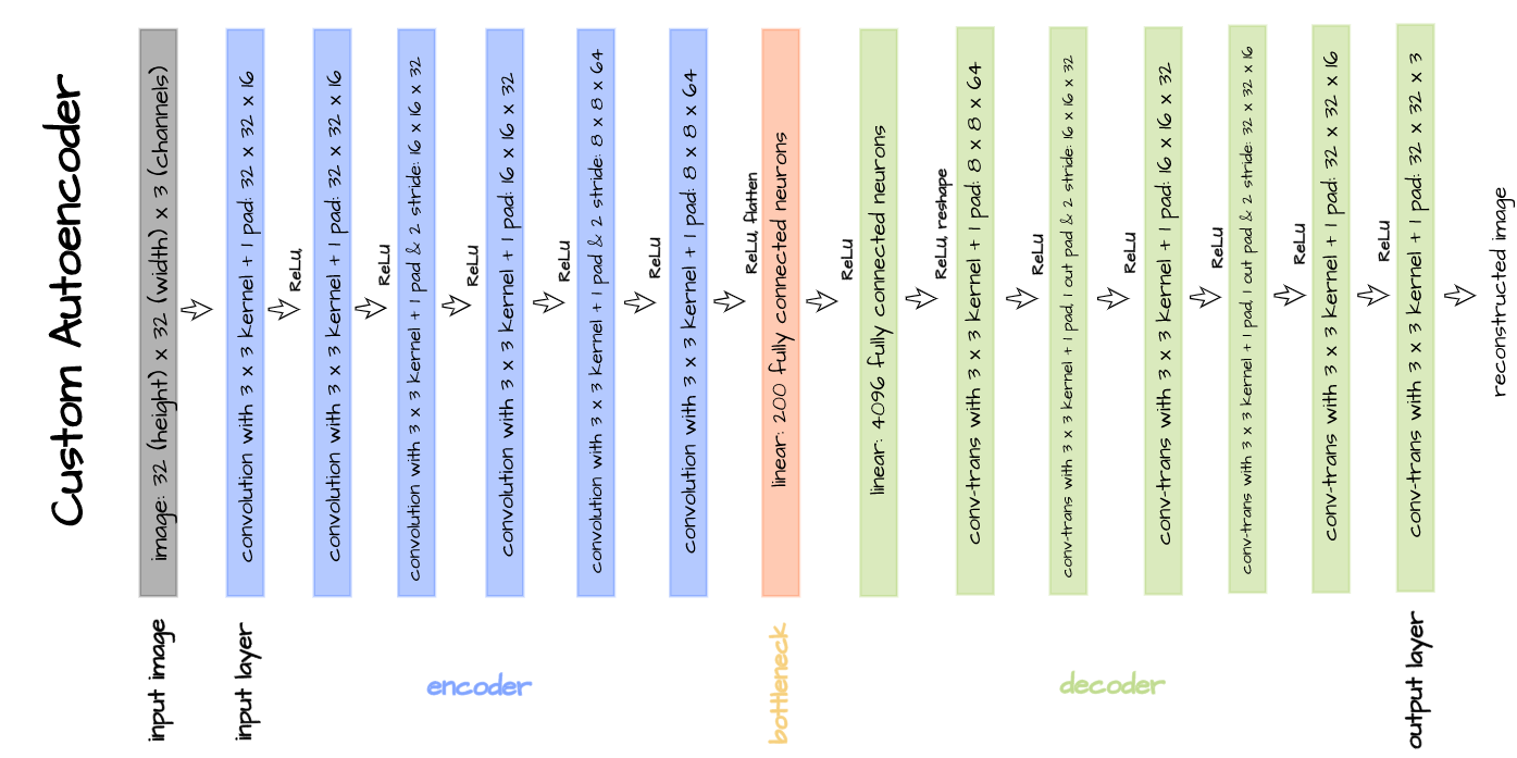
The autoencoder structure pictured above is applied within the code block beneath and can be used for coaching functions. This autoencoder is customized constructed only for illustration functions and is particularly tailor-made to the CIFAR-10 dataset. A bottleneck dimension of 1000 is used for this specific article as an alternative of 200.

#  defining encoder
class Encoder(nn.Module):
  def __init__(self, in_channels=3, out_channels=16, latent_dim=1000, act_fn=nn.ReLU()):
    tremendous().__init__()

    self.web = nn.Sequential(
        nn.Conv2d(in_channels, out_channels, 3, padding=1), # (32, 32)
        act_fn,
        nn.Conv2d(out_channels, out_channels, 3, padding=1), 
        act_fn,
        nn.Conv2d(out_channels, 2*out_channels, 3, padding=1, stride=2), # (16, 16)
        act_fn,
        nn.Conv2d(2*out_channels, 2*out_channels, 3, padding=1),
        act_fn,
        nn.Conv2d(2*out_channels, 4*out_channels, 3, padding=1, stride=2), # (8, 8)
        act_fn,
        nn.Conv2d(4*out_channels, 4*out_channels, 3, padding=1),
        act_fn,
        nn.Flatten(),
        nn.Linear(4*out_channels*8*8, latent_dim),
        act_fn
    )

  def ahead(self, x):
    x = x.view(-1, 3, 32, 32)
    output = self.web(x)
    return output


#  defining decoder
class Decoder(nn.Module):
  def __init__(self, in_channels=3, out_channels=16, latent_dim=1000, act_fn=nn.ReLU()):
    tremendous().__init__()

    self.out_channels = out_channels

    self.linear = nn.Sequential(
        nn.Linear(latent_dim, 4*out_channels*8*8),
        act_fn
    )

    self.conv = nn.Sequential(
        nn.ConvTranspose2d(4*out_channels, 4*out_channels, 3, padding=1), # (8, 8)
        act_fn,
        nn.ConvTranspose2d(4*out_channels, 2*out_channels, 3, padding=1, 
                           stride=2, output_padding=1), # (16, 16)
        act_fn,
        nn.ConvTranspose2d(2*out_channels, 2*out_channels, 3, padding=1),
        act_fn,
        nn.ConvTranspose2d(2*out_channels, out_channels, 3, padding=1, 
                           stride=2, output_padding=1), # (32, 32)
        act_fn,
        nn.ConvTranspose2d(out_channels, out_channels, 3, padding=1),
        act_fn,
        nn.ConvTranspose2d(out_channels, in_channels, 3, padding=1)
    )

  def ahead(self, x):
    output = self.linear(x)
    output = output.view(-1, 4*self.out_channels, 8, 8)
    output = self.conv(output)
    return output


#  defining autoencoder
class Autoencoder(nn.Module):
  def __init__(self, encoder, decoder):
    tremendous().__init__()
    self.encoder = encoder
    self.encoder.to(system)

    self.decoder = decoder
    self.decoder.to(system)

  def ahead(self, x):
    encoded = self.encoder(x)
    decoded = self.decoder(encoded)
    return decoded

Convolutional Autoencoder Class

In order to neatly package deal mannequin coaching and utilization right into a single object, a convolutional autoencoder class is outlined as seen beneath. This class has utilization strategies reminiscent of autoencode which facilitates the complete autoencoding course of, encode which triggers the encoder and bottleneck returning a 1000 ingredient vector encoding and decode which takes a 1000 ingredient vector as enter and makes an attempt to reconstruct a picture.

class ConvolutionalAutoencoder():
  def __init__(self, autoencoder):
    self.community = autoencoder
    self.optimizer = torch.optim.Adam(self.community.parameters(), lr=1e-3)

  def prepare(self, loss_function, epochs, batch_size, 
            training_set, validation_set, test_set):
    
    #  creating log
    log_dict = {
        'training_loss_per_batch': [],
        'validation_loss_per_batch': [],
        'visualizations': []
    } 

    #  defining weight initialization perform
    def init_weights(module):
      if isinstance(module, nn.Conv2d):
        torch.nn.init.xavier_uniform_(module.weight)
        module.bias.knowledge.fill_(0.01)
      elif isinstance(module, nn.Linear):
        torch.nn.init.xavier_uniform_(module.weight)
        module.bias.knowledge.fill_(0.01)

    #  initializing community weights
    self.community.apply(init_weights)

    #  creating dataloaders
    train_loader = DataLoader(training_set, batch_size)
    val_loader = DataLoader(validation_set, batch_size)
    test_loader = DataLoader(test_set, 10)

    #  setting convnet to coaching mode
    self.community.prepare()
    self.community.to(system)

    for epoch in vary(epochs):
      print(f'Epoch {epoch+1}/{epochs}')
      train_losses = []

      #------------
      #  TRAINING
      #------------
      print('coaching...')
      for pictures in tqdm(train_loader):
        #  zeroing gradients
        self.optimizer.zero_grad()
        #  sending pictures to system
        pictures = pictures.to(system)
        #  reconstructing pictures
        output = self.community(pictures)
        #  computing loss
        loss = loss_function(output, pictures.view(-1, 3, 32, 32))
        #  calculating gradients
        loss.backward()
        #  optimizing weights
        self.optimizer.step()

        #--------------
        # LOGGING
        #--------------
        log_dict['training_loss_per_batch'].append(loss.merchandise())

      #--------------
      # VALIDATION
      #--------------
      print('validating...')
      for val_images in tqdm(val_loader):
        with torch.no_grad():
          #  sending validation pictures to system
          val_images = val_images.to(system)
          #  reconstructing pictures
          output = self.community(val_images)
          #  computing validation loss
          val_loss = loss_function(output, val_images.view(-1, 3, 32, 32))

        #--------------
        # LOGGING
        #--------------
        log_dict['validation_loss_per_batch'].append(val_loss.merchandise())


      #--------------
      # VISUALISATION
      #--------------
      print(f'training_loss: {spherical(loss.merchandise(), 4)} validation_loss: {spherical(val_loss.merchandise(), 4)}')

      for test_images in test_loader:
        #  sending take a look at pictures to system
        test_images = test_images.to(system)
        with torch.no_grad():
          #  reconstructing take a look at pictures
          reconstructed_imgs = self.community(test_images)
        #  sending reconstructed and pictures to cpu to permit for visualization
        reconstructed_imgs = reconstructed_imgs.cpu()
        test_images = test_images.cpu()

        #  visualisation
        imgs = torch.stack([test_images.view(-1, 3, 32, 32), reconstructed_imgs], 
                          dim=1).flatten(0,1)
        grid = make_grid(imgs, nrow=10, normalize=True, padding=1)
        grid = grid.permute(1, 2, 0)
        plt.determine(dpi=170)
        plt.title('Authentic/Reconstructed')
        plt.imshow(grid)
        log_dict['visualizations'].append(grid)
        plt.axis('off')
        plt.present()
      
    return log_dict

  def autoencode(self, x):
    return self.community(x)

  def encode(self, x):
    encoder = self.community.encoder
    return encoder(x)
  
  def decode(self, x):
    decoder = self.community.decoder
    return decoder(x)

With every part setup, the autoencoder can now be skilled by instantiating it, and calling the prepare methodology with parameters as seen beneath.

#  coaching mannequin
mannequin = ConvolutionalAutoencoder(Autoencoder(Encoder(), Decoder()))

log_dict = mannequin.prepare(nn.MSELoss(), epochs=15, batch_size=64, 
                       training_set=training_data, validation_set=validation_data,
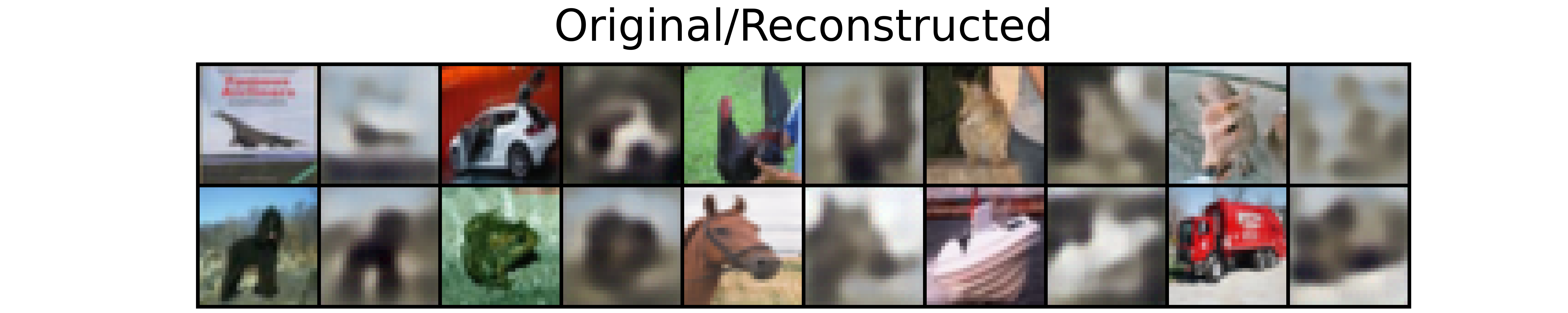
                       test_set=test_data)

After the primary epoch, we are able to see that the autoencoder has started to be taught representations robust sufficient to have the ability to put collectively enter pictures albeit with out a lot element.

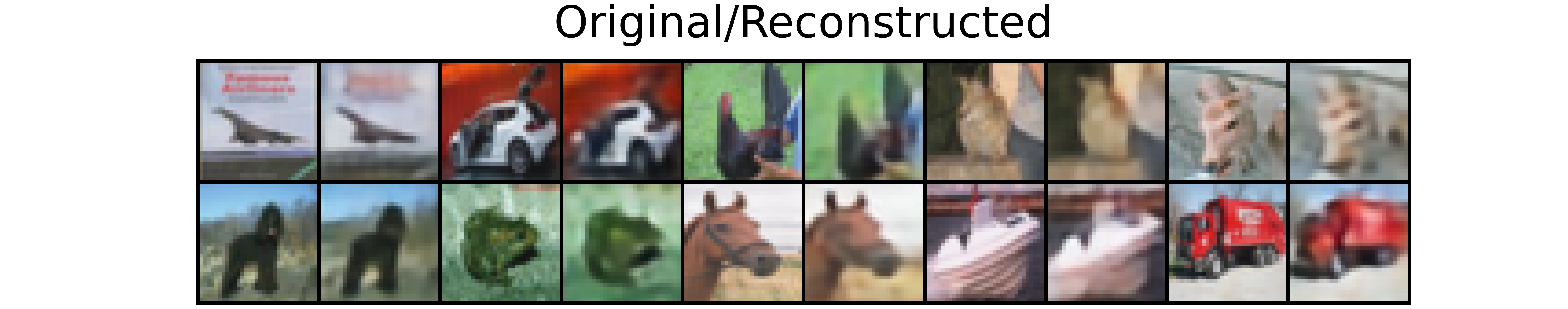
Nonetheless, by the fifteenth epoch the autoencoder has started to place collectively enter pictures in additional element with correct colours and higher kind.

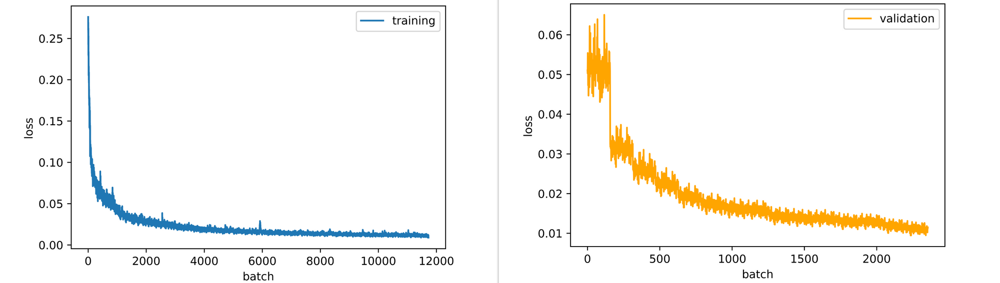
Wanting on the coaching and validation loss plots, each plots are down-trending,  and, due to this fact, the mannequin will the truth is profit from extra epochs of coaching. Nonetheless, for this text coaching for 15 epochs is deemed adequate sufficient.

Writing a Visible Similarity Perform

Now, that an autoencoder has been skilled to reconstruct pictures of all 10 courses within the CIFAR-10 dataset, we are able to proceed to make use of the autoencoder’s encoder as a characteristic extractor for any set of pictures after which examine extracted options utilizing cosine similarity.

In our case, let’s write a perform able to receiving any picture as enter after which it appears by a set of pictures (we can be utilizing the validation set for this function) for related pictures. The perform is outlined beneath as described; care have to be taken to preprocess the enter picture simply as coaching pictures had been preprocessed since that is what the mannequin expects.

def visual_similarity(filepath, mannequin, dataset, options):
  """
  This perform replicates the visible similarity course of
  as outlined beforehand.
  """
  #  studying picture
  picture = cv2.imread(filepath)
  picture = cv2.cvtColor(picture, cv2.COLOR_BGR2RGB)
  picture = cv2.resize(picture, (32, 32))

  #  changing picture to tensor/preprocessing picture
  my_transforms=transforms.Compose([transforms.ToTensor(),
                                    transforms.Normalize((0.5, 0.5, 0.5), (0.5, 0.5, 0.5))])
  picture = my_transforms(picture)

  #  encoding picture
  picture = picture.to(system)
  with torch.no_grad():
    image_encoding = mannequin.encode(picture)

  #  computing similarity scores
  similarity_scores = [F.cosine_similarity(image_encoding, x) for x in features]
  similarity_scores = [x.cpu().detach().item() for x in similarity_scores]
  similarity_scores = [round(x, 3) for x in similarity_scores]
 
  #  creating pandas collection
  scores = pd.Collection(similarity_scores)
  scores = scores.sort_values(ascending=False)

  #  deriving probably the most related picture
  idx = scores.index[0]
  most_similar = [image, dataset[idx]]

  #  visualization
  grid = make_grid(most_similar, normalize=True, padding=1)
  grid = grid.permute(1,2,0)
  plt.determine(dpi=100)
  plt.title('uploaded/most_similar')
  plt.axis('off')
  plt.imshow(grid)

  print(f'similarity rating = {scores[idx]}')
  go

Since we’re going to be evaluating the uploaded picture to pictures within the validation set we might save time by extracting options from all 1000 pictures previous to utilizing the perform. This course of would as effectively have been written into the similarity perform however it should come on the expense of compute time. That is carried out beneath.

#  extracting options from pictures within the validation set
with torch.no_grad():
  image_features = [model.encode(x.to(device)) for x in tqdm_regular(validation_data)]

Computing Similarity

On this part, some pictures can be equipped to the visible similarity perform in a bid to entry the outcomes produced. It needs to be borne in thoughts nonetheless that solely pictures in courses current within the coaching set will produce cheap outcomes.  

Picture 1

Contemplate the picture of a German Shepard with a white background as seen beneath. This canine is has a predominantly golden coat with a black saddle and it’s noticed to be standing at alert going through the left.  

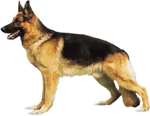
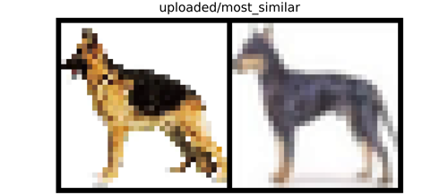
Upon passing this picture to the visible similarity perform, a plot of the uploaded picture in opposition to probably the most related picture within the validation set is produced. Notice that the unique picture was downsized to 32 x 32 pixels as required by the mannequin.

visual_similarity('image_1.jpg', mannequin=mannequin, 
                  dataset=validation_data, 
                  options=image_features)

From the end result, a white background picture of a seemingly darkish coat canine standing at alert going through the left is returned with a similarity rating of 92.2%. On this case, the mannequin primarily finds a picture which matches a lot of the particulars of the unique which is strictly what we would like.

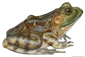
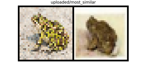
Picture 2

The picture beneath is that of a typically brownish trying frog in a inclined place going through the rightward path on a white background. Once more, passing the picture by our visible similarity perform produces a plot of the uploaded picture in opposition to it is most related picture.

visual_similarity('image_2.jpg', mannequin=mannequin, 
                  dataset=validation_data, 
                  options=image_features)

From the ensuing plot, a considerably grey trying frog in an identical place (inclined) to our uploaded picture is returned with a similarity rating of about 91%. Discover that the picture can also be depicted on a white background.

Picture 3

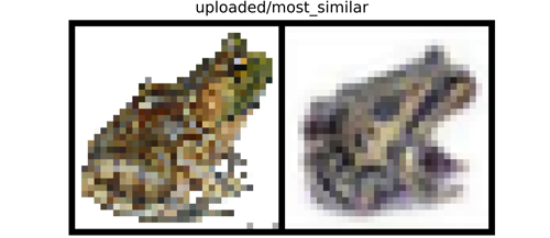
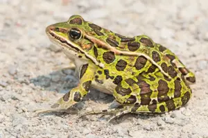
Lastly, beneath we’ve got a picture of one other frog. This frog is of greenish coloration in a equally inclined place to the frog within the earlier picture however with distinctions of going through the leftward path and being depicted on a textured background (sand on this case).

visual_similarity('image_3.jpg', mannequin=mannequin, 
                  dataset=validation_data, 
                  options=image_features)

Similar to within the earlier two sections, when the picture is equipped to the visible similarity perform a plot of the unique picture and probably the most related picture discovered within the validation set is returned. Probably the most related picture on this case is that of a brownish trying frog in a inclined place, going through the leftward path, depicted on a textured background as effectively. A similarity rating of roughly 90% is returned.

From the photographs used as examples on this part it may be seen that the visible similarity perform works because it ought to. Nonetheless, with extra epochs of coaching or maybe a greater structure, there’s a chance that higher similarity suggestions can be made past the primary few most related pictures.

On this article, we had been in a position to have a look at one other helpful use of autoencoders, this time as a device for visible similarity advice. Right here we explored how an autoencoder’s encoder can be utilized as a characteristic extractor with the extracted options then in contrast utilizing cosine similarity to be able to discover related pictures.

Mainly all of the autoencoder does on this occasion is to extract options. Certainly, in case you are fairly conversant with convolutional neural networks, then you’ll agree that not solely autoencoders might function characteristic extractors, however that networks used for classification functions is also used for characteristic extraction. Thus, this means their utility for visible similarity duties in flip.