

Convey this venture to life
Typically instances, deep studying fashions are stated to be black boxed in nature. Black boxed within the sense that their outputs are troublesome to clarify or some instances merely unexplainable. Nevertheless, there are some Python libraries which assist to supply some form of rationalization to the output of deep studying fashions. On this article, we will probably be looking at a type of libraries: SHAP.
#  article dependencies
import torch
import torch.nn as nn
import torch.nn.purposeful as F
import torchvision
import torchvision.transforms as transforms
import torchvision.datasets as Datasets
from torch.utils.information import Dataset, DataLoader
import numpy as np
import matplotlib.pyplot as plt
import cv2
from tqdm.pocket book import tqdm
import seaborn as sns
from torchvision.utils import make_grid
!pip set up shap
import shap
if torch.cuda.is_available():
machine = torch.machine('cuda:0')
print('Working on the GPU')
else:
machine = torch.machine('cpu')
print('Working on the CPU')Mannequin Explainability
Mannequin explainability refers back to the course of whereby outputs produced by machine studying fashions are defined by way of how and which options affect the mannequin’s precise output. For example, think about a random forest mannequin educated to foretell home costs; assume that dataset the mannequin was educated on solely has 3 options, variety of bedrooms, variety of bogs and dimension of the lounge. Assume the mannequin predicts a home to be price about $300,000, with mannequin explainability we are able to derive insights on how a lot every characteristic contributes both positively or negatively to the expected worth.
Mannequin Explainability within the Context of Laptop Imaginative and prescient
As regards deep studying, pc imaginative and prescient classification duties specifically, since options are basically pixels, mannequin explainability helps to establish pixels which contribute negatively or positively to the expected class.
On this article, the SHAP library will probably be used for deep studying mannequin explainability. SHAP, quick for Shapely Additive exPlanations is a sport concept primarily based method to explaining outputs of machine studying fashions, extra info will be present in its official documentation.
Implementing Deep Studying Mannequin Explainability
On this part, we will probably be coaching a convolutional neural community for a classification process earlier than continuing to derive a perception into why the mannequin classifies an occasion of information into a selected class utilizing the SHAP library.
Dataset
The dataset for use for coaching functions as regards this text would be the CIFAR10 dataset. It is a dataset containing 32 x 32 pixel photos belonging to 10 distinct lessons starting from airplanes to horses. It may be loaded in PyTorch utilizing the code cell beneath.
#  loading coaching information
training_set = Datasets.CIFAR10(root="./", obtain=True,
                                remodel=transforms.ToTensor())

#  loading validation information
validation_set = Datasets.CIFAR10(root="./", obtain=True, practice=False,
                                  remodel=transforms.ToTensor())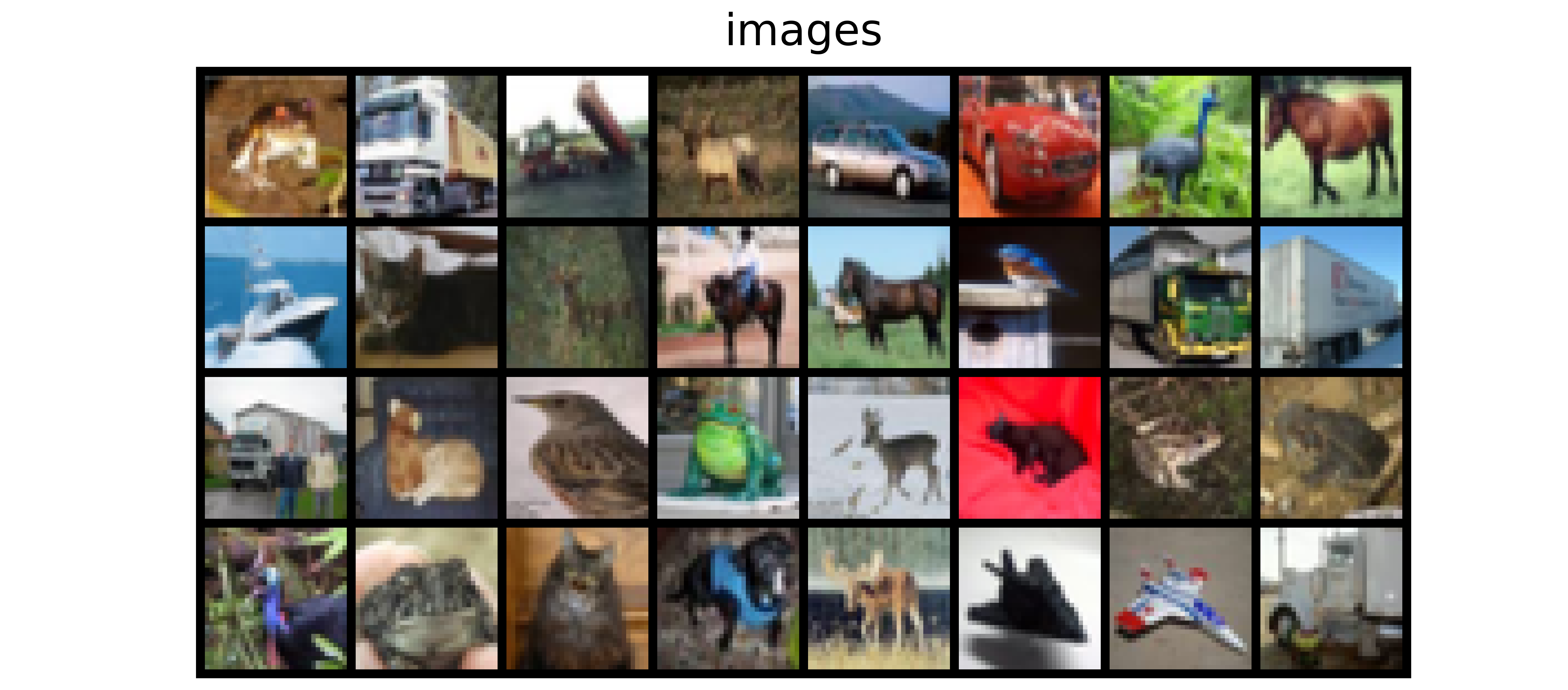
| Label | Description |
|---|---|
| 0 | Airplane |
| 1 | Car |
| 2 | Chook |
| 3 | Cat |
| 4 | Deer |
| 5 | Canine |
| 6 | Frog |
| 7 | Horse |
| 8 | Ship |
| 9 | Truck |
Mannequin Structure
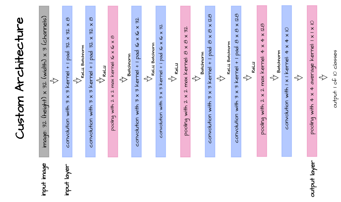
The mannequin structure as illustrated above is carried out within the following code cell. It is a customized structure designed purposefully for the sake of this text. This structure takes in 32 x 32 pixel photos and is comprised of seven convolutional layers.
class ConvNet(nn.Module):
  def __init__(self):
    tremendous().__init__()
    self.conv1 = nn.Conv2d(3, 8, 3, padding=1)
    self.batchnorm1 = nn.BatchNorm2d(8)
    self.conv2 = nn.Conv2d(8, 8, 3, padding=1)
    self.batchnorm2 = nn.BatchNorm2d(8)
    self.pool2 = nn.MaxPool2d(2)
    self.conv3 = nn.Conv2d(8, 32, 3, padding=1)
    self.batchnorm3 = nn.BatchNorm2d(32)
    self.conv4 = nn.Conv2d(32, 32, 3, padding=1)
    self.batchnorm4 = nn.BatchNorm2d(32)
    self.pool4 = nn.MaxPool2d(2)
    self.conv5 = nn.Conv2d(32, 128, 3, padding=1)
    self.batchnorm5 = nn.BatchNorm2d(128)
    self.conv6 = nn.Conv2d(128, 128, 3, padding=1)
    self.batchnorm6 = nn.BatchNorm2d(128)
    self.pool6 = nn.MaxPool2d(2)
    self.conv7 = nn.Conv2d(128, 10, 1)
    self.pool7 = nn.AvgPool2d(3)

  def ahead(self, x):
    #-------------
    # INPUT
    #-------------
    x = x.view(-1, 3, 32, 32)

    #-------------
    # LAYER 1
    #-------------
    output_1 = self.conv1(x)
    output_1 = F.relu(output_1)
    output_1 = self.batchnorm1(output_1)

    #-------------
    # LAYER 2
    #-------------
    output_2 = self.conv2(output_1)
    output_2 = F.relu(output_2)
    output_2 = self.pool2(output_2)
    output_2 = self.batchnorm2(output_2)

    #-------------
    # LAYER 3
    #-------------
    output_3 = self.conv3(output_2)
    output_3 = F.relu(output_3)
    output_3 = self.batchnorm3(output_3)

    #-------------
    # LAYER 4
    #-------------
    output_4 = self.conv4(output_3)
    output_4 = F.relu(output_4)
    output_4 = self.pool4(output_4)
    output_4 = self.batchnorm4(output_4)

    #-------------
    # LAYER 5
    #-------------
    output_5 = self.conv5(output_4)
    output_5 = F.relu(output_5)
    output_5 = self.batchnorm5(output_5)

    #-------------
    # LAYER 6
    #-------------
    output_6 = self.conv6(output_5)
    output_6 = F.relu(output_6)
    output_6 = self.pool6(output_6)
    output_6 = self.batchnorm6(output_6)

    #--------------
    # OUTPUT LAYER
    #--------------
    output_7 = self.conv7(output_6)
    output_7 = self.pool7(output_7)
    output_7 = output_7.view(-1, 10)

    return F.softmax(output_7, dim=1)
Convolutional Neural Community Class
To be able to neatly put collectively our mannequin, we are going to write a category which encompasses each coaching, validation and mannequin utilization into one object as seen beneath.
class ConvolutionalNeuralNet():
  def __init__(self, community):
    self.community = community.to(machine)
    self.optimizer = torch.optim.Adam(self.community.parameters(), lr=1e-3)

  def practice(self, loss_function, epochs, batch_size,
            training_set, validation_set):

    #  creating log
    log_dict = {
        'training_loss_per_batch': [],
        'validation_loss_per_batch': [],
        'training_accuracy_per_epoch': [],
        'training_recall_per_epoch': [],
        'training_precision_per_epoch': [],
        'validation_accuracy_per_epoch': [],
        'validation_recall_per_epoch': [],
        'validation_precision_per_epoch': []
    }

    #  defining weight initialization operate
    def init_weights(module):
      if isinstance(module, nn.Conv2d):
        torch.nn.init.xavier_uniform_(module.weight)
        module.bias.information.fill_(0.01)
      elif isinstance(module, nn.Linear):
        torch.nn.init.xavier_uniform_(module.weight)
        module.bias.information.fill_(0.01)

    #  defining accuracy operate
    def accuracy(community, dataloader):
      community.eval()

      all_predictions = []
      all_labels = []

      #  computing accuracy
      total_correct = 0
      total_instances = 0
      for photos, labels in tqdm(dataloader):
        photos, labels = photos.to(machine), labels.to(machine)
        all_labels.prolong(labels)
        predictions = torch.argmax(community(photos), dim=1)
        all_predictions.prolong(predictions)
        correct_predictions = sum(predictions==labels).merchandise()
        total_correct+=correct_predictions
        total_instances+=len(photos)
      accuracy = spherical(total_correct/total_instances, 3)

      #  computing recall and precision
      true_positives = 0
      false_negatives = 0
      false_positives = 0
      for idx in vary(len(all_predictions)):
        if all_predictions[idx].merchandise()==1 and  all_labels[idx].merchandise()==1:
          true_positives+=1
        elif all_predictions[idx].merchandise()==0 and all_labels[idx].merchandise()==1:
          false_negatives+=1
        elif all_predictions[idx].merchandise()==1 and all_labels[idx].merchandise()==0:
          false_positives+=1
      strive:
        recall = spherical(true_positives/(true_positives + false_negatives), 3)
      besides ZeroDivisionError:
        recall = 0.0
      strive:
        precision = spherical(true_positives/(true_positives + false_positives), 3)
      besides ZeroDivisionError:
        precision = 0.0
      return accuracy, recall, precision

    #  initializing community weights
    self.community.apply(init_weights)

    #  creating dataloaders
    train_loader = DataLoader(training_set, batch_size)
    val_loader = DataLoader(validation_set, batch_size)

    #  setting convnet to coaching mode
    self.community.practice()

    for epoch in vary(epochs):
      print(f'Epoch {epoch+1}/{epochs}')
      train_losses = []

      #  coaching
      print('coaching...')
      for photos, labels in tqdm(train_loader):
        #  sending information to machine
        photos, labels = photos.to(machine), labels.to(machine)
        #  resetting gradients
        self.optimizer.zero_grad()
        #  making predictions
        predictions = self.community(photos)
        #  computing loss
        loss = loss_function(predictions, labels)
        log_dict['training_loss_per_batch'].append(loss.merchandise())
        train_losses.append(loss.merchandise())
        #  computing gradients
        loss.backward()
        #  updating weights
        self.optimizer.step()
      with torch.no_grad():
        print('deriving coaching accuracy...')
        #  computing coaching accuracy
        train_accuracy, train_recall, train_precision = accuracy(self.community, train_loader)
        log_dict['training_accuracy_per_epoch'].append(train_accuracy)
        log_dict['training_recall_per_epoch'].append(train_recall)
        log_dict['training_precision_per_epoch'].append(train_precision)

      #  validation
      print('validating...')
      val_losses = []

      #  setting convnet to analysis mode
      self.community.eval()

      with torch.no_grad():
        for photos, labels in tqdm(val_loader):
          #  sending information to machine
          photos, labels = photos.to(machine), labels.to(machine)
          #  making predictions
          predictions = self.community(photos)
          #  computing loss
          val_loss = loss_function(predictions, labels)
          log_dict['validation_loss_per_batch'].append(val_loss.merchandise())
          val_losses.append(val_loss.merchandise())
        #  computing accuracy
        print('deriving validation accuracy...')
        val_accuracy, val_recall, val_precision = accuracy(self.community, val_loader)
        log_dict['validation_accuracy_per_epoch'].append(val_accuracy)
        log_dict['validation_recall_per_epoch'].append(val_recall)
        log_dict['validation_precision_per_epoch'].append(val_precision)

      train_losses = np.array(train_losses).imply()
      val_losses = np.array(val_losses).imply()

      print(f'training_loss: {spherical(train_losses, 4)}  training_accuracy: '+
      f'{train_accuracy}  training_recall: {train_recall}  training_precision: {train_precision} *~* validation_loss: {spherical(val_losses, 4)} '+
      f'validation_accuracy: {val_accuracy}  validation_recall: {val_recall}  validation_precision: {val_precision}n')

    return log_dict

  def predict(self, x):
    return self.community(x)
Mannequin Coaching
Convey this venture to life
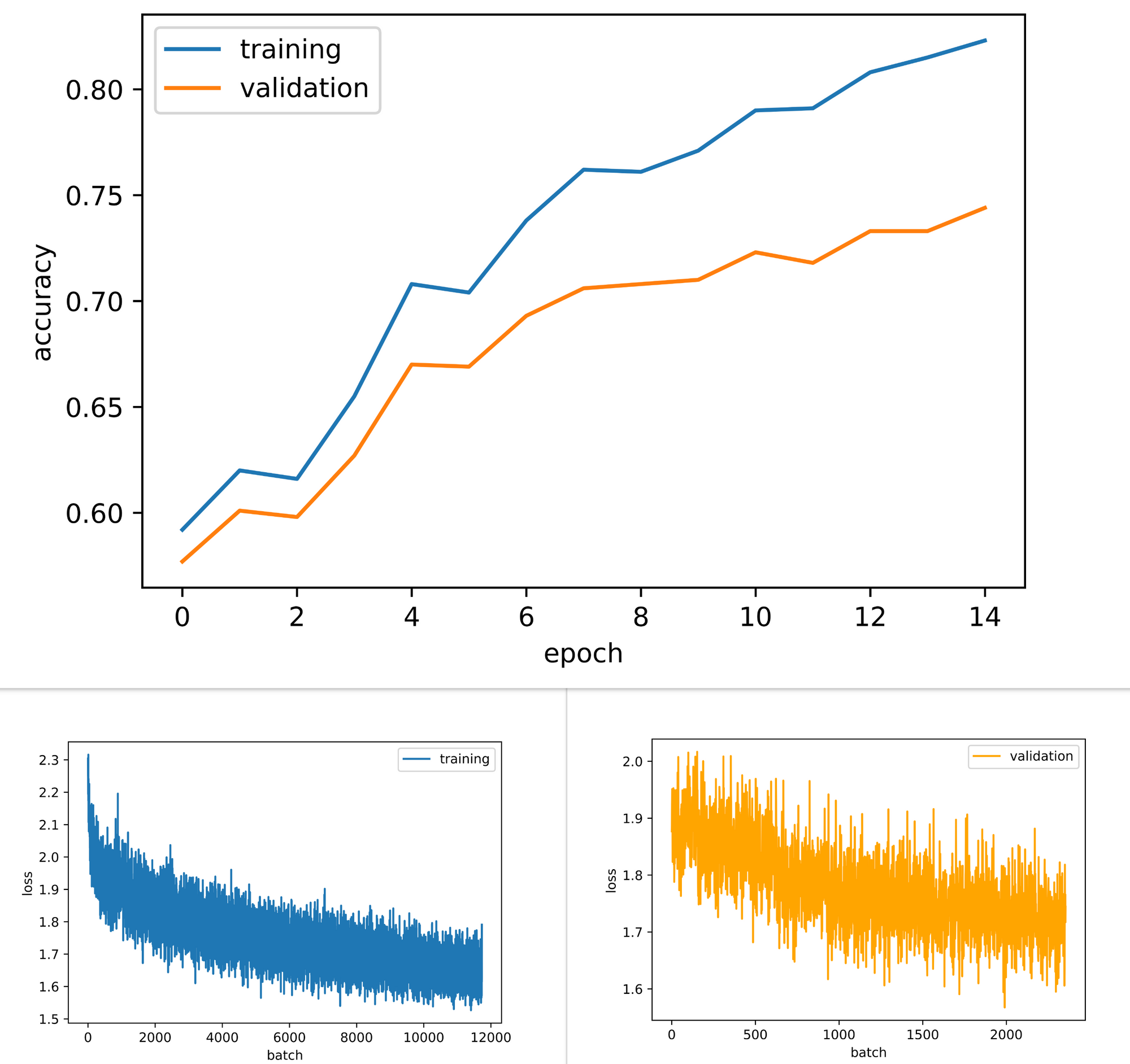
With the whole lot setup, it is now time to coach the mannequin. Utilizing parameters as outlined, the mannequin is educated for 15 epochs.
mannequin = ConvolutionalNeuralNet(ConvNet())

log_dict = mannequin.practice(nn.CrossEntropyLoss(), epochs=15, batch_size=64,
                       training_set=training_set, validation_set=validation_set)
From outcomes obtained, each coaching and validation accuracy elevated via the course of mannequin coaching. Validation accuracy attained a worth just below 75%, not the perfect performing mannequin however will suffice for this text’s aims. Moreover, each coaching and validation losses are down-trending indicative of higher efficiency being obtained with extra epochs of coaching.
Mannequin Explainability
On this part we will probably be making an attempt to clarify/derive insights into the classifications made by the mannequin educated within the earlier part. As talked about beforehand, we will probably be utilizing the SHAP library for this objective.
Principally, the library does this by using the mannequin in classifying a few cases in a bid to know its habits and the character of its outputs, this ‘understanding’ known as the explainer. Afterwards, utilizing the article containing the explainer, values are then assigned to every characteristic (pixels on this case) which influences the classification made by the mannequin, these values are termed SHAP values. These SHAP values are the precise metrics which indicate explainability; primarily based on the magnitude of those values one can develop an thought into how every pertinent characteristic has contributed to the classification made by the mannequin. Lastly, a plot known as a SHAP plot is produced to make interpretation of the aforementioned values simpler.
Making a Masks
As talked about beforehand, to be able to generate SHAP values an explainer has to have been generated prior. This explainer makes classification on some information cases, these information cases are known as a masks. For this text, the primary 200 cases within the validation set are chosen because the masks. There are thereafter transformed right into a PyTorch dataset by instantiating them as a member of the CustomMask class.
#  defining dataset class
class CustomMask(Dataset):
  def __init__(self, information, transforms=None):
    self.information = information
    self.transforms = transforms

  def __len__(self):
    return len(self.information)

  def __getitem__(self, idx):
    picture = self.information[idx]

    if self.transforms!=None:
      picture = self.transforms(picture)
    return picture

#  creating explainer masks
masks = validation_set.information[:200]

#  turning masks to pytorch dataset
masks = CustomMask(masks, transforms=transforms.ToTensor())
Explainability Operate
All of the steps outlined above can then be put collectively to supply a operate which implements mannequin explainability by producing SHAP plots for any occasion of information categorised by the mannequin.
The operate beneath does particularly that. Firstly, it takes in parameters comparable to a picture in array type, a masks and a deep studying mannequin. Subsequent the picture array is transformed to a tensor and classification is made earlier than mapping the classification vector output to a dictionary of labels native to CIFAR10.
Thereafter, an explainer is derived from the masks and mannequin equipped earlier than SHAP values are produced for the picture of selection utilizing this explainer. A SHAP plot is then returned for straightforward interpretation.
def plot_shap(image_array, masks, mannequin):
  """
  This operate performs mannequin explainability
  by producing shap plots for a knowledge occasion
  """
  #  changing picture to tensor
  picture = transforms.ToTensor()(image_array)
  picture = picture.to(machine)

  #-----------------
  #  CLASSIFICATION
  #-----------------
  #  making a mapping of lessons to labels
  label_dict = {0:'airplane', 1:'car', 2:'hen', 3:'cat', 4:'deer',
                5:'canine', 6:'frog', 7:'horse', 8:'ship', 9:'truck'}

  #  using the mannequin for classification
  with torch.no_grad():
    prediction = torch.argmax(mannequin(picture), dim=1).merchandise()

  #  displaying mannequin classification
  print(f'prediction: {label_dict[prediction]}')

  #----------------
  #  EXPLANABILITY
  #----------------
  #  creating dataloader for masks
  mask_loader = DataLoader(masks, batch_size=200)

  #  creating explainer for mannequin behaviour
  for photos in mask_loader:
    photos = photos.to(machine)
    explainer = shap.DeepExplainer(mannequin, photos)
    break

  #  deriving shap values for picture of curiosity primarily based on mannequin behaviour
  shap_values = explainer.shap_values(picture.view(-1, 3, 32, 32))

  #  getting ready for visualization by altering channel association
  shap_numpy = [np.swapaxes(np.swapaxes(x, 1, -1), 1, 2) for x in shap_values]
  image_numpy = np.swapaxes(np.swapaxes(picture.view(-1, 3, 32, 32).cpu().numpy(), 1, -1), 1, 2)

  #  producing shap plots
  shap.image_plot(shap_numpy, image_numpy, present=False, labels= ['airplane', 'automobile', 'bird',
                                                                'cat', 'deer', 'dog','frog',
                                                                'horse', 'ship', 'truck'])
  go
Understanding SHAP Plots
Using the operate written above we are able to then start to develop an understanding of why the mannequin classifies an occasion of information because it has. For a fast and straightforward demonstration, we are able to merely use photos within the validation set as seen within the code cell beneath.
plot_shap(validation_set.information[-150], masks, mannequin.community)
Kind the output returned, the mannequin accurately predicts this picture occasion as a Horse. The following SHAP plot consists of the unique picture adopted by 10 dim grayscale variations of itself. Every grayscale picture is indicative of particular person lessons within the dataset and is labeled as such. Beneath the plot is a scale which reads from unfavorable to optimistic, shade coded from deep blue to vibrant pink. This scale helps to point out the depth of the SHAP worth assigned to every pertinent pixel.
Pixels coloured deep blue are these which push the mannequin away from predicting that the picture belongs to that exact class whereas pixels coloured vibrant pink are these which strongly point out that the picture in all probability belongs to the category in query; white coloration then again present that no significance was positioned on these pixels by the mannequin. Shades of colours in-between these talked about range proportionally.
Taking one other take a look at the plot above it may be seen that the mannequin has narrowed down it is gaze on two lessons for that exact occasion of information, Deer and Horse. In each lessons, there are related patterns of pink pixels on the high of the picture which means that objects in that a part of the picture are synonymous to photographs of Deers and Horses (ie most Deers and Horses within the coaching set are pictured on a woodland background as seen in that information occasion). Nevertheless, pixels alongside the place of the article of curiosity signifies that the Horse class possesses extra pink pixels compared to the Deer class. Which means that the mannequin has perceived that the form of that object is extra synonymous with that of a Horse.
Instance 2

Contemplate the picture occasion above, once more derived from the validation set. This picture is accurately categorised as a Deer however trying on the SHAP plots, one can see that the mannequin had a harder time deciding which class the picture belongs to when in comparison with the earlier picture. All the lessons are lit up with pink and blue pixels on this case with lessons car, hen and truck much less lit than others.
The lessons cat, deer, canine, frog and horse have essentially the most exercise on their grayscales, significantly on their backgrounds because it appears a major variety of the photographs in these lessons contained within the coaching set are pictured on grass backgrounds. Nevertheless, the mannequin has categorised the picture as a Deer since there are much less blue pixels general in comparison with the opposite lessons.
Instance 3

Not like the opposite two photos, this information occasion which is evidently a canine was misclassified as an airplane. On the floor this would possibly look like a fairly weird classification however trying on the SHAP plots extra mild is shed on why the mannequin behaved this fashion.
From the plot, each the airplane and the canine class have been assumed to be most probably. Nevertheless, distinctive variations are seen within the nature of SHAP values alongside the perimeters of the grayscales because the ear and neck area of the canine is usually blue on airplane and pink on canine, whereas areas alongside the outstretched ft of canine are lit pink on airplane and blue on canine.
What this means is that whereas the mannequin acknowledges that the pinnacle and neck area of the picture is most probably that of a canine, the truth that the canine is in a stretched out place implies an aerodynamic form which is most typical in airplanes. It’s most probably that there will not be many photos of canine in that place within the coaching set for the mannequin to correctly study that distinction.
Utilizing Imported Pictures
By extending the operate written within the earlier part, we are able to make it so it receives an uploaded picture, makes predictions after which present mannequin explainability by way of a SHAP plot. That is performed beneath.
def plot_shap_util(filepath, masks, mannequin):
  """
  This operate performs mannequin explainability
  by producing shap plots for a knowledge occasion
  """
  #  studying picture and changing to tensor
  picture = cv2.imread(filepath)
  picture = cv2.cvtColor(picture, cv2.COLOR_BGR2RGB)
  picture = cv2.resize(picture, (32, 32))
  picture = transforms.ToTensor()(picture)
  picture = picture.to(machine)

  #-----------------
  #  CLASSIFICATION
  #-----------------
  #  making a mapping of lessons to labels
  label_dict = {0:'airplane', 1:'car', 2:'hen', 3:'cat', 4:'deer',
                5:'canine', 6:'frog', 7:'horse', 8:'ship', 9:'truck'}

  #  using the mannequin for classification
  prediction = torch.argmax(mannequin(picture), dim=1).merchandise()

  #  displaying mannequin classification
  print(f'prediction: {label_dict[prediction]}')

  #----------------
  #  EXPLANABILITY
  #----------------
  #  creating dataloader for masks
  mask_loader = DataLoader(masks, batch_size=200)

  #  creating explainer for mannequin behaviour
  for photos in mask_loader:
    photos = photos.to(machine)
    explainer = shap.DeepExplainer(mannequin, photos)
    break

  #  deriving shap values for picture of curiosity primarily based on mannequin behaviour
  shap_values = explainer.shap_values(picture.view(-1, 3, 32, 32))

  #  getting ready for visualization by altering channel association
  shap_numpy = [np.swapaxes(np.swapaxes(x, 1, -1), 1, 2) for x in shap_values]
  test_numpy = np.swapaxes(np.swapaxes(picture.view(-1, 3, 32, 32).cpu().numpy(), 1, -1), 1, 2)

  #  producing shap plots
  shap.image_plot(shap_numpy, test_numpy, present=False, labels= ['airplane', 'automobile', 'bird', 'cat', 'deer',
                                                               'dog', 'frog', 'horse', 'ship', 'truck'])

  go
Utilizing the prolonged operate, we are able to then provide photos as parameter and classification will probably be offered, adopted by a SHAP plot which might then be interpreted for explainability.
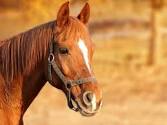
#  utilizing the prolonged explainability operate
plot_shap_util('picture.jpg', masks, mannequin.community)
On this case, the mannequin has accurately categorised the uploaded picture as that of a Horse because it has much less of blue pixels and extra of pink pixels in comparison with different lessons. Although on this case, a localized area alongside the bottom of the picture appear to play an enormous function on this classification which is troublesome to decipher.
Mannequin explainability helps to supply some helpful perception into why a mannequin behaves the best way it does regardless that not all explanations might make sense or be simple to interpret. SHAP is only one strategy to clarify outputs of deep studying fashions there exist quite a few different libraries that can be utilized to the identical impact.
Notice: For this text, higher explanations will be gotten with a greater mannequin. A greater mannequin within the context of higher structure and higher mannequin efficiency, be happy to vary the mannequin structure or practice the mannequin for extra epochs if deemed vital.