Ensembling Neural Network Models With Tensorflow

Mannequin ensembling is a standard follow in machine studying to enhance the efficiency and generalizability of fashions.  It may be merely described because the method of mixing a number of fashions in various methods to enhance efficiency on a single drawback.

The main deserves of mannequin ensembling embrace its capacity to enhance the efficiency, robustness and generalization of machine studying fashions on unseen information.

Tree-based algorithms are significantly identified to carry out higher for sure duties attributable to their capacity to make the most of the ensembling of a number of timber to enhance the mannequin’s general efficiency.

The ensemble members ( i.e fashions which can be mixed to a single mannequin or prediction) are mixed utilizing various aggregation strategies comparable to easy or weighted averaging to different superior strategies comparable to bagging, stacking or boosting.

In distinction to classical algorithms, it is not a standard for a number of neural community fashions to be ensembled for a single activity. That is largely as a result of single fashions are sometimes sufficient to map the connection between options and targets and ensembling a number of neural networks may complicate the mannequin for smaller duties and result in overfitting of the mannequin. It is commonest for practitioners to extend the scale of a single neural community mannequin to correctly match the information than ensemble a number of neural community fashions into one.

Nonetheless, for bigger duties, ensembling a number of neural networks, particularly ones skilled on comparable issues, may show fairly helpful and enhance the efficiency of the ultimate mannequin and its capacity to generalize on broader use instances.

Oftentimes, practitioners check out a number of fashions with completely different configurations to pick out the best-performing mannequin for an issue. Neural community ensembling provides the choice of using the data of the completely different fashions to develop a extra balanced and environment friendly mannequin.

For instance, combining a number of community fashions that had been skilled on a specific dataset (such because the Imagenet dataset) may show helpful to enhance the efficiency of a mannequin being skilled on a dataset with comparable lessons. The completely different data realized by the fashions may very well be mixed by mannequin ensembling to enhance the mannequin’s general efficiency and robustness of an aggregated mannequin. Earlier than ensembling such fashions, it is very important practice and fine-tune the ensemble members to make sure that every mannequin contributes related data to the ultimate mannequin.

The Tensorflow API supplies sure strategies for aggregating a number of community fashions utilizing built-in community layers or by constructing customized layers.

On this tutorial, we ensemble customized and pre-trained community fashions which can be skilled on comparable datasets utilizing customized and built-in Tensorflow layers to strategy a picture classification drawback. We might ensemble our fashions utilizing concatenation, common and weighted common ensembling strategies.

This goals to function a template of various strategies for combining a number of community fashions in your tasks.

The Dataset

Our use case is a picture classification of pure photographs. We might be utilizing the Pure Photos Dataset which comprises 6899 photographs of pure photographs representing 8 lessons. The represented lessons within the dataset are aeroplane, automotive, cat, canine, fruit, motorcycle and particular person.

Our intention is to develop a neural community mannequin that’s able to figuring out photographs belonging to the completely different lessons and precisely classifying new photographs of every class.

Workflow

We might develop three completely different fashions for our activity after which ensemble utilizing completely different strategies. You will need to configure our fashions to supply related data to our ultimate mannequin.

Seed the atmosphere for reproducibility and preview a number of the photographs within the dataset representing every class.

# Seed atmosphere 
seed_value = 1 # seed worth 

# Set`PYTHONHASHSEED` atmosphere variable at a set worth 
import os os.environ['PYTHONHASHSEED']=str(seed_value) 

# Set the `python` built-in pseudo-random generator at a set worth 
import random 
random.seed = seed_value 

# Set the `numpy` pseudo-random generator at a set worth 
import numpy as np 
np.random.seed = seed_value 

# Set the `tensorflow` pseudo-random generator at a set worth import tensorflow as tf tf.seed = seed_value

Set the information configurations and get the lessons

# set configs 
base_path="./natural_images" 
target_size = (224,224,3) 

# outline form for all photographs # get lessons lessons = os.listdir(base_path) print(lessons)

Plot Pattern photographs of the dataset

# plot pattern photographs 

import matplotlib.pyplot as plt
import cv2

f, axes = plt.subplots(2, 4, sharex=True, sharey=True, figsize = (16,7))

for ax, label in zip(axes.ravel(), lessons):
    img = np.random.alternative(os.listdir(os.path.be a part of(base_path, label)))
    img = cv2.imread(os.path.be a part of(base_path, label, img))
    img = cv2.resize(img, target_size[:2])
    ax.imshow(cv2.cvtColor(img, cv2.COLOR_BGRA2RGB))
    ax.set_title(label)
    ax.axis(False)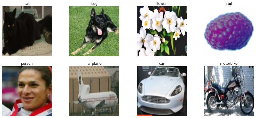

‌Load the photographs.

We load the photographs in batches utilizing the Keras Picture Generator and specify a validation cut up to separate the dataset into coaching and validation splits.

We additionally apply random picture augmentation to increase the coaching dataset so as to enhance the efficiency of the mannequin and its capacity to generalize.

from keras.preprocessing.picture import ImageDataGenerator

batch_size = 32

datagen = ImageDataGenerator(rescale=1./255,
                                   rotation_range=20,
                                   shear_range=0.2,
                                   zoom_range=0.2,
                                   width_shift_range = 0.2,
                                   height_shift_range = 0.2,
                                   vertical_flip = True,
                                   validation_split=0.25)

train_gen = datagen.flow_from_directory(base_path,
                                               target_size=target_size[:2],
                                               batch_size=batch_size,
                                               class_mode="categorical",
                                               subset="coaching")
val_gen =  datagen.flow_from_directory(base_path,
                                               target_size=target_size[:2],
                                               batch_size=batch_size,
                                               class_mode="categorical",
                                               subset="validation",
                                               shuffle=False)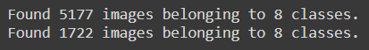

1. Construct and practice a customized mannequin.‌

For our first mannequin, we construct a customized mannequin utilizing the Tensorflow purposeful technique

# Construct mannequin 
enter = Enter(form= target_size) 

x = Conv2D(filters=32, kernel_size=(3,3), activation='relu')(enter) 
x = MaxPool2D(2,2)(x) 

x = Conv2D(filters=64, kernel_size=(3,3), activation='relu')(x) 
x = MaxPool2D(2,2)(x) 

x = Conv2D(filters=128, kernel_size=(3,3), activation='relu')(x) 
x = MaxPool2D(2,2)(x) 

x = Conv2D(filters=256, kernel_size=(3,3), activation='relu')(x) 
x = MaxPool2D(2,2)(x) 

x = Dropout(0.25)(x) 
x = Flatten()(x) 
x = Dense(models=128, activation='relu')(x) 
x = Dense(models=64, activation='relu')(x) 
output = Dense(models=8, activation='softmax')(x) 

custom_model  = Mannequin(enter, output, title="Custom_Model")

Subsequent, we compile the customized mannequin and initialize the callbacks to watch and management coaching. For our callback, we scale back the training fee when there isn’t a enchancment for a couple of epochs, we initialize EarlyStopping to cease the coaching course of if the mannequin doesn’t additional enhance and in addition checkpoint the coaching to save lots of our greatest mannequin at every epoch. These are helpful normal practices for coaching deep studying fashions.

# compile mannequin
custom_model.compile(loss="categorical_crossentropy", optimizer="rmsprop", metrics=['accuracy']) 

# initialize callbacks 
reduceLR = ReduceLROnPlateau(monitor="val_loss", persistence= 3, verbose= 1,                                  mode="min", issue=  0.2, min_lr = 1e-6) 

early_stopping = EarlyStopping(monitor="val_loss", persistence = 5 , verbose=1,                                  mode="min", restore_best_weights= True) 

checkpoint = ModelCheckpoint('CustomModel.weights.hdf5', monitor="val_loss",                               verbose=1,save_best_only=True, mode="min") 

callbacks= [reduceLR, early_stopping,checkpoint]

Now we are able to outline our coaching configurations and practice our customized mannequin.

# outline coaching config 
TRAIN_STEPS = 5177 // batch_size 
VAL_STEPS = 1722 //batch_size 
epochs = 80 

# practice mannequin
custom_model.match(train_gen, steps_per_epoch= TRAIN_STEPS, validation_data=val_gen, validation_steps=VAL_STEPS, epochs= epochs, callbacks= callbacks)

After coaching our customized mannequin we are able to consider the mannequin’s efficiency. I shall be evaluating the mannequin on the validation set. In follow, it’s preferable to put aside a separate take a look at set for mannequin analysis.

# Consider the mannequin 
custom_model.consider(val_gen)

‌We will additionally retrieve the prediction and precise validation labels in order to verify the classification report and confusion matrix evaluations for the customized mannequin.

# get validation labels
val_labels = [] 
for i in vary(VAL_STEPS + 1):
  val_labels.prolong(val_gen[i][1])

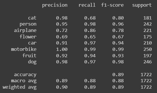
val_labels = np.argmax(val_labels, axis=1)

# present classification report 

from sklearn.metrics import classification_report 

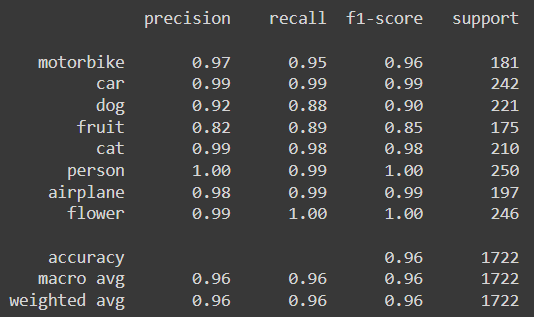
print(classification_report(val_labels, predicted_labels, target_names=lessons))

# operate to plot confusion matrix

import itertools

def plot_confusion_matrix(precise, predicted):

    cm = confusion_matrix(precise, predicted)
    cm = cm.astype('float') / cm.sum(axis=1)[:, np.newaxis]

    plt.determine(figsize=(7,7))
    cmap=plt.cm.Blues
    plt.imshow(cm, interpolation='nearest', cmap=cmap)
    plt.title('Confusion matrix', fontsize=25)
  
    tick_marks = np.arange(len(lessons))
    plt.xticks(tick_marks, lessons, rotation=90, fontsize=15)
    plt.yticks(tick_marks, lessons, fontsize=15)

    thresh = cm.max() / 2.
    for i, j in itertools.product(vary(cm.form[0]), vary(cm.form[1])):
        plt.textual content(j, i, format(cm[i, j], '.2f'),
        horizontalalignment="middle",
        coloration="white" if cm[i, j] > thresh else "black", fontsize = 14)

    plt.ylabel('True label', fontsize=20)
    plt.xlabel('Predicted label', fontsize=20)
    plt.present()

# plot confusion matrix
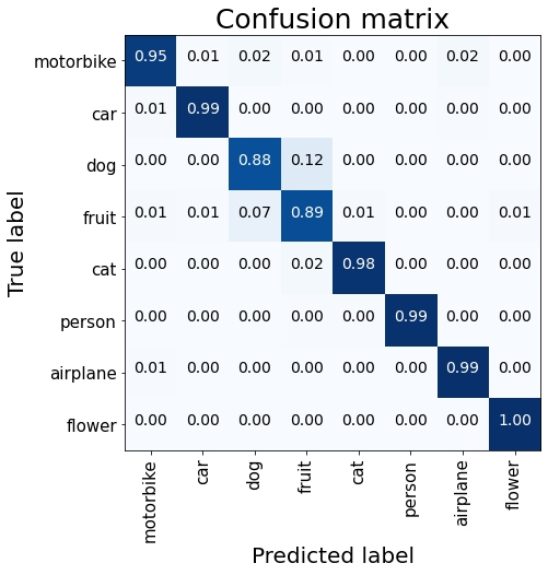
plot_confusion_matrix(val_labels, predicted_labels)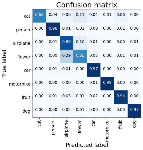

From the mannequin analysis, we discover that the customized mannequin couldn’t correctly establish the photographs of cats and flowers. It additionally provides sub-optimal precision for figuring out aeroplanes.

Subsequent, we’d check out a special model-building method, by utilizing weights realized by networks pre-trained on the Imagenet dataset to spice up our mannequin’s efficiency within the lessons with decrease accuracy scores.

2. Utilizing a pre-trained VGG16 mannequin.

for our second mannequin ,we’d be utilizing the VGG16 mannequin pre-trained on the Imagenet dataset to coach a mannequin for our use case. This enables us to inherit the weights realized from coaching on the same dataset to spice up our mannequin’s efficiency.

Initializing and fine-tuning the VGG16 mannequin.

# Import the VGG16 pretrained mannequin 
from tensorflow.keras.purposes import VGG16 

# initialize the mannequin vgg16 = VGG16(input_shape=(224,224,3), weights="imagenet", include_top=False) 

# Freeze all however the final 3 layers for layer in vgg16.layers[:-3]: layer.trainable = False 

# construct mannequin 
enter = vgg16.layers[-1].output # enter is the final output from vgg16 

x = Dropout(0.25)(enter) 
x = Flatten()(x) 
output = Dense(8, activation='softmax')(x) 

# create the mannequin 
vgg16_model = Mannequin(vgg16.enter, output, title="VGG16_Model")

We initialize the pre-trained mannequin and freeze all however the final three layers so we are able to make the most of the weights of the fashions and be taught new data within the final 3 layers which can be particular to our use case. We additionally add a dropout layer to regularize the mannequin from overfitting on our dataset earlier than including our ultimate output layer.

We will then practice our VGG16 fine-tuned mannequin utilizing comparable coaching configurations to our customized mannequin.

# compile the mannequin 
vgg16_model.compile(optimizer= SGD(learning_rate=1e-3), loss="categorical_crossentropy", metrics= ['accuracy']) 

# reinitialize callbacks 
checkpoint = ModelCheckpoint('VggModel.weights.hdf5', monitor="val_loss", verbose=1,save_best_only=True, mode="min") 

callbacks= [reduceLR, early_stopping,checkpoint] 

# Prepare mannequin 
vgg16_model.match(train_gen, steps_per_epoch= TRAIN_STEPS, validation_data=val_gen, validation_steps=VAL_STEPS, epochs= epochs, callbacks= callbacks)

After coaching, we are able to consider the mannequin’s efficiency utilizing comparable scripts from the final mannequin analysis.

# Consider the mannequin 
vgg16_model.consider(val_gen)

# get the mannequin predictions 
predicted_labels = np.argmax(vgg16_model.predict(val_gen), axis=1) 

# present classification report 
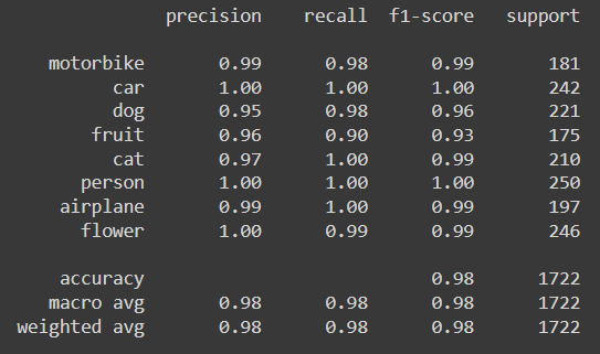
print(classification_report(val_labels, predicted_labels, target_names=lessons)) 

# plot confusion matrix 
plot_confusion_matrix(val_labels, predicted_labels)

Utilizing a pre-trained VGG16 mannequin produced higher efficiency, particularly for the lessons with decrease scores.

Lastly, earlier than ensembling, we’d use one other pre-trained mannequin with a lot lesser parameters than the VGG16. The intention is to make the most of completely different architectures so we are able to profit from their various properties to enhance the standard of our ultimate mannequin. We might be utilizing the Mobilenet mannequin pre-trained on the identical Imagenet dataset.

3. Utilizing a pre-trained Mobilenet mannequin.

For our ultimate mannequin, we’d be finetuning the mobilenet mannequin

# initializing the mobilenet mannequin
mobilenet = MobileNet(input_shape=(224,224,3), weights="imagenet", include_top=False)

# freezing all however the final 5 layers
for layer in mobilenet.layers[:-5]:
  layer.trainable = False

# add few mor layers
x = mobilenet.layers[-1].output
x = Dropout(0.5)(x)
x = Flatten()(x) 
x = Dense(32, activation='relu')(x)
x = Dropout(0.5)(x)
x = Dense(16, activation='relu')(x)
output = Dense(8, activation='softmax')(x)

# Create the mannequin
mobilenet_model = Mannequin(mobilenet.enter, output, title= "Mobilenet_Model")

For coaching the mannequin, we keep a number of the earlier configurations from our earlier coaching.

# compile the mannequin 
mobilenet_model.compile(optimizer= SGD(learning_rate=1e-3), loss="categorical_crossentropy", metrics= ['accuracy']) 

# reinitialize callbacks 
checkpoint = ModelCheckpoint('MobilenetModel.weights.hdf5', monitor="val_loss", verbose=1,save_best_only=True, mode="min") 

callbacks= [reduceLR, early_stopping,checkpoint] 

# mannequin coaching 
mobilenet_model.match(train_gen, steps_per_epoch= TRAIN_STEPS, validation_data=val_gen, validation_steps=VAL_STEPS, epochs=epochs, callbacks= callbacks)

After coaching our fine-tuned Mobilenet mannequin, we are able to then consider its efficiency.

# Consider the mannequin 
mobilenet_model.consider(val_gen) 

# get the mannequin's predictions 
predicted_labels = np.argmax(mobilenet_model.predict(val_gen), axis=1) 

# present the classification report 
print(classification_report(val_labels, predicted_labels, target_names=lessons)) 

# plot the confusion matrix 
plot_confusion_matrix(val_labels, predicted_labels)

The fine-tuned Mobilenet mannequin performs higher than the earlier fashions and notably improves the identification of canine and flowers.

Whereas it might be wonderful to make use of the skilled Mobilenet mannequin or any of our fashions as our ultimate alternative, combining the construction and weights of the three fashions may show higher in growing a single, extra generalizable mannequin in manufacturing.

Ensembling The Fashions

To ensemble the fashions, we’d be utilizing three completely different ensembling strategies as earlier acknowledged: Concatenation, Common and Weighted Common.

The strategies have their professionals and cons which are sometimes thought of to find out the selection for a specific use case.

Concatenation Ensemble

This includes merging the parameters of a number of fashions right into a single mannequin. That is made doable in Tensorflow by the concatenation layer which receives inputs of tensors of the identical form (aside from the concatenation axis) and merges them into one. This layer can due to this fact be used to merge all the data learnt by the completely different fashions facet by facet on a single axis right into a single mannequin. See right here for extra details about the Tensorflow concatenation layer.

To merge our fashions, we’d merely enter our fashions into the concatenation layer.

# concatenate the fashions

# import concatenate layer
from tensorflow.keras.layers import Concatenate

# get checklist of fashions
fashions = [custom_model, vgg16_model, mobilenet_model] 

enter = Enter(form=(224, 224, 3), title="enter") # enter layer

# get output for every mannequin enter
outputs = [model(input) for model in models]

# contenate the ouputs
x = Concatenate()(outputs) 

# add additional layers
x = Dropout(0.5)(x) 
output = Dense(8, activation='softmax', title="output")(x) # output layer

# create concatenated mannequin
conc_model = Mannequin(enter, output, title="Concatenated_Model")

After concatenation, we added additional layers as deemed acceptable for our activity. On this instance, I’ve added a dropout layer and a ultimate output layer with the suitable output dimensions of our use case.

Let’s verify the construction of our concatenated mannequin.

# present mannequin construction 
from tensorflow.keras.utils import plot_model 
plot_model(conc_model)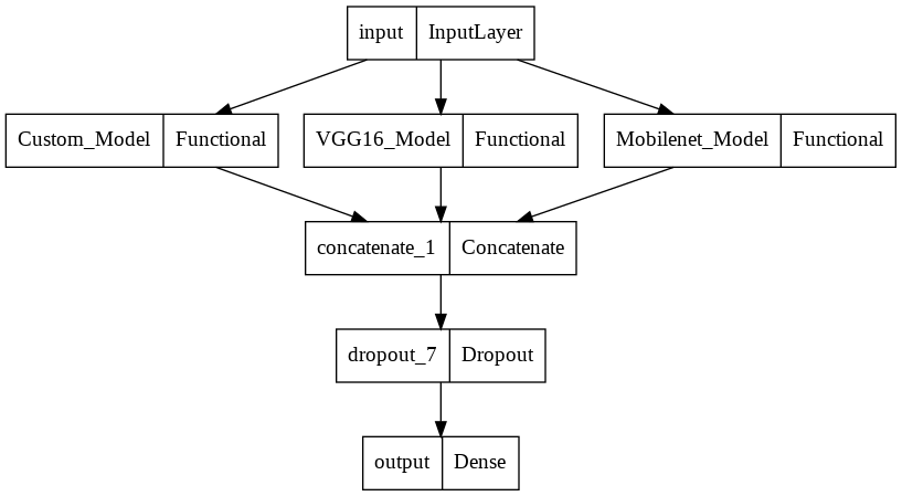

We will see how the three completely different purposeful fashions we have constructed are merged into one with additional dropout and output layers.

This might show helpful for sure instances as we’re using all the data gained by the completely different fashions. The issue with this technique is that the dimension of our ultimate mannequin is a concatenation of the scale of all of the ensemble members which may result in a dimensionality explosion, the inclusion of irrelevant data and consequently, overfitting.

Common Ensemble

Slightly than danger exploding the mannequin’s dimension and overfitting for easier duties by concatenating a number of fashions, we may merely make our ultimate mannequin the typical of all our fashions. This fashion, we’re capable of keep an affordable common dimension for our ultimate mannequin whereas using the data of all our fashions.

This time we are going to use the Tensorflow Common layer which receives inputs and outputs their common. Subsequently our ultimate mannequin is a median of the parameters of our enter fashions. See right here for extra details about the typical layer.

To ensemble our mannequin by common,  we merely mix our fashions on the common layer.

# common ensemble mannequin 

# import Common layer
from tensorflow.keras.layers import Common 

enter = Enter(form=(224, 224, 3), title="enter")  # enter layer

# get output for every enter mannequin
outputs = [model(input) for model in models] 

# take common of the outputs
x = Common()(outputs) 

x = Dense(16, activation='relu')(x) 
x = Dropout(0.3)(x) 
output = Dense(8, activation='softmax', title="output")(x) # output layer

# create common ensembled mannequin
avg_model = Mannequin(enter, output)

As beforehand seen,  additional layers may be added to the community as deemed match. We will additionally see the construction of the Common ensembled mannequin.

# present mannequin construction 
plot_model(avg_model)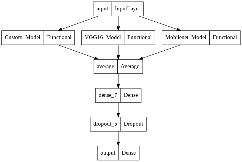

This strategy to ensembling is especially helpful as a result of by taking a median, the decrease efficiency for sure lessons is boosted by fashions with greater efficiency for such lessons, thereby bettering the mannequin’s general efficiency and generalization.

The draw back to this strategy is that by taking the typical, sure data from the fashions wouldn’t be included within the ultimate mannequin. One other is that as a result of we’re taking a easy common, the prevalence and relevance of sure fashions are misplaced. As in our use case, the prevalence in efficiency of the Mobilenet Mannequin over different fashions is misplaced.

This may very well be resolved by taking a weighted common of the fashions when ensembling, such that it displays the significance of every mannequin to the ultimate determination.

Weighted Common Ensemble

In weighted common ensembling, the outputs of the fashions are multiplied by an assigned weight and a median is taken to get a ultimate mannequin.  By assigning weights to the fashions when ensembling this fashion, we protect their significance and contribution to the ultimate determination.

Whereas TensorFlow doesn’t have a built-in layer for weighted common ensembling, we may make the most of attributes of the built-in Layer class to implement a customized weighted common ensemble layer. For a weighted common ensemble, it’s obligatory that the weights sum as much as one, we are able to guarantee this by making use of a softmax operate on the weights earlier than ensembling. You possibly can see extra about creating customized layers in TensorFlow right here.

Implementing a customized weighted common layer

First, we outline a customized operate to set our weights.

# operate for setting weights

import numpy as np

def weight_init(form =(1,1,3), weights=[1,2,3], dtype=tf.float32):
    return tf.fixed(np.array(weights).reshape(form), dtype=dtype)

Right here we have now set a weight of 1,2 and three for our fashions respectively. We will then construct our customized weighted common layer.

# implement customized weighted common layer

import tensorflow as tf
from tensorflow.keras.layers import Layer, Concatenate

class WeightedAverage(Layer):

    def __init__(self):
        tremendous(WeightedAverage, self).__init__()
        
    def construct(self, input_shape):
        
        self.W = self.add_weight(
                    form=(1,1,len(input_shape)),
                    initializer=weighted_init,
                    dtype=tf.float32,
                    trainable=True)
    def name(self, inputs):
    
        inputs = [tf.expand_dims(i, -1) for i in inputs]
        inputs = Concatenate(axis=-1)(inputs) 
        weights = tf.nn.softmax(self.W, axis=-1)

        return tf.reduce_mean(weights*inputs, axis=-1)
    

To construct our customized weighted common layer, we inherited attributes of the built-in Layer class and added weights utilizing our weights initializing operate. We apply a softmax to our initialized weights in order that they sum as much as one earlier than multiplying it with the fashions.  Lastly, we get the imply discount of the weighted inputs to get our ultimate mannequin.

We will then ensemble our mannequin utilizing the customized weighted common layer.

enter = Enter(form=(224, 224, 3), title="enter")  # enter layer

# get output for every enter mannequin
outputs = [model(input) for model in models] 

# get weighted common of outputs
x = WeightedAverage()(outputs)

output = Dense(8, activation='softmax')(x) # output layer

weighted_avg_model = Mannequin(enter, output, title="Weighted_AVerage_Model")

Let’s verify the construction of our weighted common mannequin.

# plot mannequin
plot_model(weighted_avg_model)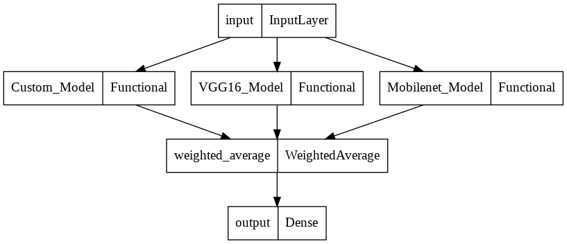

As within the earlier strategies, our fashions are ensembled, however this time, as a weighted common of the three fashions. The output dimension of the ensembled mannequin can be suitable with the required output dimension for our activity with out including any additional layers.

Additionally, relatively than manually set our weights utilizing a customized weight initializing operate, we may additionally make the most of Tensorflow built-in weight initializers to initialize weights which can be optimized throughout coaching. See right here for the obtainable built-in weight initializers in Tensorflow.

Abstract

Mannequin ensembling supplies strategies of mixing a number of fashions to spice up the efficiency and generalization of machine studying fashions. Neural networks may be mixed utilizing Tensorflow by concatenation, common or customized weighted common strategies. All the data from the ensemble members is preserved utilizing the concatenation method on the danger of dimension explosion. Utilizing the typical technique maintains an affordable dimension for our mannequin however loses sure data and doesn’t account for the significance of every contributing mannequin. This may be resolved by utilizing a customized weighted common with weights which can be optimized in the course of the coaching course of. There’s additionally the potential of extending  Neural Community ensembling utilizing different operations.