Implementation of ProGAN from scratch

ProGAN from the paper Progressive Rising of GANs for Improved High quality, Stability, and Variation is among the revolutionary papers that was the primary to generate actually high-quality photographs. On this article, we are going to make a clear, easy, and readable implementation of it utilizing PyTorch. (Should you favor TensorFlow/Keras you possibly can see this superb article written by Bharath Okay.)  We are going to attempt to replicate the unique paper as intently as potential, so in case you learn the paper the implementation ought to be just about similar.

Should you do not learn the ProGan paper or do not know the way it works and also you wish to perceive it I extremely suggest you to take a look at this publish weblog the place I am going throw the main points of it. And if you’re new to GANs you can begin with this text the place I clarify why GANs are superior, perceive what GANs actually are, how they work, dive deep into the loss perform that they use, after which construct a easy GAN from scratch to generate MNIST.

The dataset that we are going to use on this weblog is that this dataset from Kaggle which incorporates 16240 higher garments for ladies with 256*192 decision. It is actually a small dataset with low decision in comparison with the one which the authors of ProGAN use which incorporates 800k photographs with excessive decision 1024*1024 nevertheless it nonetheless provides us good outcomes. You possibly can attempt to use a greater dataset to get better-generated photographs of any variety you need (faces, automobiles, homes,…).

Now let’s begin by loading the mandatory libraries.

Load all dependencies we’d like

We first will import torch since we are going to use PyTorch, and from there we import nn. That can assist us create and prepare the networks, and in addition allow us to import optim, a package deal that implements varied optimization algorithms (e.g. sgd, adam,..). From torchvision we import datasets and transforms to arrange the information and apply some transforms.

We are going to import useful as F from torch.nn to upsample the photographs utilizing interpolate, DataLoader from torch.utils.knowledge to create mini-batch sizes, save_image from torchvision.utils to avoid wasting faux samples, and log2 type math as a result of we’d like the inverse illustration of the ability of two to implement the adaptive minibatch dimension relying on the output decision, Numpy for linear algebra, os for interplay with the working system, tqdm to indicate progress bars, and at last matplotlib.pyplot to indicate the outcomes and evaluate them with the true ones.

import torch
from torch import nn, optim
from torchvision import datasets, transforms
import torch.nn.useful as F
from torch.utils.knowledge import DataLoader
from torchvision.utils import save_image
from math import log2
import numpy as np
import os
from tqdm import tqdm
import matplotlib.pyplot as plt

Seed every thing

Let’s seed every thing to make outcomes considerably reproducible

def seed_everything(seed=42):
    os.environ['PYTHONHASHSEED'] = str(seed)
    np.random.seed(seed)
    torch.manual_seed(seed)
    torch.cuda.manual_seed(seed)
    torch.cuda.manual_seed_all(seed)
    torch.backends.cudnn.deterministic = True
    torch.backends.cudnn.benchmark = False
seed_everything()

Hyperparameters

• Initialize the DATASET by the trail of the true photographs.
• Specify the beginning prepare at picture dimension 4 by 4 because the paper.
• Initialize the gadget by Cuda whether it is out there and CPU in any other case, and studying price by 0.001.
• The batch dimension might be totally different relying on the decision of the photographs that we wish to generate, so we initialize BATCH_SIZES by an inventory of numbers, you possibly can change them relying in your VRAM.
• Initialize image_size by 128 and CHANNELS_IMG by 3 as a result of we are going to generate 128  by 128 RGB photographs.
• Within the unique paper, they initialize Z_DIM and IN_CHANNELS by 512, however I initialize them by 256 as an alternative for much less VRAM utilization and speed-up coaching. We may even perhaps get higher outcomes if we doubled them.
• For ProGAN we are able to use any of the GANs loss features we would like however we want to observe the paper precisely, so we are going to use the identical loss perform as they used the Wasserstein loss perform, also called WGAN-GP from the paper Improved Coaching of Wasserstein GANs. This loss incorporates a parameter identify λ and it is common to set λ = 10.
• Initialize PROGRESSIVE_EPOCHS by 30 for every picture dimension.

DATASET                 = "Girls garments"
START_TRAIN_AT_IMG_SIZE = 4
DEVICE                  = "cuda" if torch.cuda.is_available() else "cpu"
LEARNING_RATE           = 1e-3
BATCH_SIZES             = [32, 32, 32, 16, 16, 16] #you should utilize [32, 32, 32, 16, 16, 16, 16, 8, 4] for instance if you wish to prepare till 1024x1024, however once more this numbers rely in your vram
image_size              = 128
CHANNELS_IMG            = 3
Z_DIM                   = 256  # ought to be 512 in unique paper
IN_CHANNELS             = 256  # ought to be 512 in unique paper
LAMBDA_GP               = 10
PROGRESSIVE_EPOCHS      = [30] * len(BATCH_SIZES)

Get and verify the Information loader

Now let’s create a perform get_loader to:

• Apply some transformation to the photographs (resize the photographs to the decision that we would like, convert them to tensors, then apply some augmentation, and at last normalize them to be all of the pixels starting from -1 to 1).
• Determine the present batch dimension utilizing the record BATCH_SIZES, and take as an index the integer variety of the inverse illustration of the ability of two of image_size/4. And that is really how we implement the adaptive minibatch dimension relying on the output decision.
• Put together the dataset we use ImageFolder as a result of it is already structured in a pleasant means.
• Create mini-batch sizes utilizing DataLoader that take the dataset and batch dimension with shuffling the information.
• Lastly, return the loader and dataset.

def get_loader(image_size):
    remodel = transforms.Compose(
        [
            transforms.Resize((image_size, image_size)),
            transforms.ToTensor(),
            transforms.RandomHorizontalFlip(p=0.5),
            transforms.Normalize(
                [0.5 for _ in range(CHANNELS_IMG)],
                [0.5 for _ in range(CHANNELS_IMG)],
            ),a
        ]
    )
    batch_size = BATCH_SIZES[int(log2(image_size / 4))]
    dataset = datasets.ImageFolder(root=DATASET, remodel=remodel)
    loader = DataLoader(
        dataset,
        batch_size=batch_size,
        shuffle=True,
    )
    return loader, dataset

Now let’s verify if every thing works superb and see what the true photographs seem like.

def check_loader():
    loader,_ = get_loader(128)
    fabric ,_ = subsequent(iter(loader))
    _, ax    = plt.subplots(3,3, figsize=(8,8))
    plt.suptitle('Some actual samples', fontsize=15, fontweight="daring")
    ind = 0 
    for ok in vary(3):
        for kk in vary(3):
            ind += 1
            ax[k][kk].imshow((fabric[ind].permute(1,2,0)+1)/2) 
check_loader()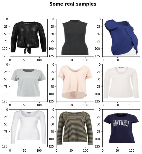

Fashions implementation

Now let’s Implement the ProGAN generator and discriminator with the important thing attributions from the paper. We are going to attempt to make the implementation compact but in addition preserve it readable and comprehensible. Particularly, the important thing factors:

• Progressive rising (of mannequin and layers)
• Minibatch std on Discriminator
• Normalization with PixelNorm
• Equalized Studying Fee

We clarify all these key factors intimately on this article.

Many of the difficult components are within the implementation of the fashions. So that is positively going to be the toughest a part of this tutorial, because of this I’m asking you to be just a little bit extra targeted and affected person.

Let’s start by constructing the generator.

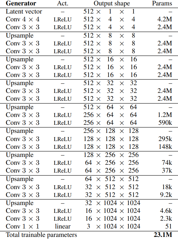
Within the determine above, we are able to see the structure of the generator. For the variety of channels, we have now 512 (256 in our case) four-time, then we lower it by 1/2, 1/4, and so forth. Let’s outline a variable with the identify elements which might be utilized in Discrmininator and Generator for the way a lot the channels ought to be multiplied and expanded for every layer.

elements = [1, 1, 1, 1, 1 / 2, 1 / 4, 1 / 8, 1 / 16, 1 / 32]

Equalized Studying Fee

Now let’s implement Equalized Studying Fee for the generator, let’s identify the category WSConv2d (weighted scaled convolutional layer) which might be inherited from nn.Module.

• Within the init half we ship in_channels, out_channels, kernel_size, stride, and padding. We use all of that to do a standard Conv layer, then we outline a scale that would be the similar because the perform part2 within the determine beneath, we copy the bias of the present column layer right into a variable as a result of we do not need the bias of the convolution layer to be scaled, then we take away it, Lastly, we initialize conv layer.  

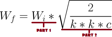
• Within the ahead half, we ship x and all that we’re going to do is multiplicate x with scale and add the bias after reshaping it.

class WSConv2d(nn.Module):

    def __init__(
        self, in_channels, out_channels, kernel_size=3, stride=1, padding=1,
    ):
        tremendous(WSConv2d, self).__init__()
        self.conv      = nn.Conv2d(in_channels, out_channels, kernel_size, stride, padding)
        self.scale     = (2 / (in_channels * (kernel_size ** 2))) ** 0.5
        self.bias      = self.conv.bias #Copy the bias of the present column layer
        self.conv.bias = None      #Take away the bias

        # initialize conv layer
        nn.init.normal_(self.conv.weight)
        nn.init.zeros_(self.bias)

    def ahead(self, x):
        return self.conv(x * self.scale) + self.bias.view(1, self.bias.form[0], 1, 1)

Normalization with PixelNorm

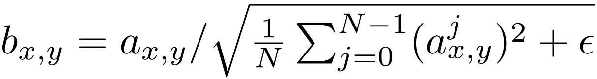
Now let’s create a category for PixelNorm, for normalization.

• Within the init half we outline epsilon by 10^-8.
• Within the ahead half, we ship x, and we return the identical because the perform within the determine beneath.

class PixelNorm(nn.Module):
    def __init__(self):
        tremendous(PixelNorm, self).__init__()
        self.epsilon = 1e-8

    def ahead(self, x):
        return x / torch.sqrt(torch.imply(x ** 2, dim=1, keepdim=True) + self.epsilon)

ConvBlock

Should you observed within the Generator structure they repeat two convolution layers with three by three filters a bunch of instances, so let’s make them in a separate class to make the code cleaner, and really, we’re going to use it within the discriminator as properly, the one distinction between the 2 is that the discriminator we is not going to use pixel norm.

• Within the init half we ship in_channels, out_channels, and use_pixelnorm, then we initialize conv1 by WSConv2d which maps in_channels to out_channels, conv2 by WSConv2d which maps out_channels to out_channels, leaky by Leaky ReLU with a slope of 0.2 as they use within the paper, pn by PixelNorm(The final block that we create), and  use_pn by use_pixelnorm to specify if we’re utilizing PixelNorm or not.
• Within the ahead half, we ship x, and we go it to conv1 with leaky, then we normalize it with pn (PixelNorm) if use_pixelnorm is True, in any other case, we do not, and once more we go that into conv2 with leaky and we normalize it if use_pixelnorm is True. Lastly, we return x.

class ConvBlock(nn.Module):
    def __init__(self, in_channels, out_channels, use_pixelnorm=True):
        tremendous(ConvBlock, self).__init__()
        self.use_pn = use_pixelnorm
        self.conv1  = WSConv2d(in_channels, out_channels)
        self.conv2  = WSConv2d(out_channels, out_channels)
        self.leaky  = nn.LeakyReLU(0.2)
        self.pn     = PixelNorm()

    def ahead(self, x):
        x = self.leaky(self.conv1(x))
        x = self.pn(x) if self.use_pn else x
        x = self.leaky(self.conv2(x))
        x = self.pn(x) if self.use_pn else x
        return x

Generator

Alright, we’re progressing very properly 😊, now let’s construct the generator.

• Should you see the primary sample within the Generator structure, you’ll discover that’s totally different than different patterns. so within the init half let’s initialize ‘preliminary’ by the layers of the primary sample, then let’s initialize ‘initial_rgb’ by WSConv2d that maps in_channels to img_channels (3 for RGB), prog_blocks by ModuleList() that can comprise all of the progressive blocks (we point out convolution enter/output channels by multiplicate in_channels which is 512 in paper and 256 in our case with elements), and rgb_blocks by ModuleList() that can comprise all of the RGB blocks.
• To fade in new layers (a part of ProGAN), we add the fade_in half, which we ship alpha, scaled, and generated, and we return  [tanh(alpha * generated +(1-alpha) * upscale)] The rationale why we use tanh is that would be the output(the generated picture) and we would like the pixels to be vary between 1 and -1.
• Within the ahead half, we ship x which is the Z_dim, the alpha worth which goes to fade in slowly throughout coaching (alpha is between 0 and 1), and steps which is the quantity of the present decision that we’re working with(steps=0 for 4×4 photographs, steps=1 for 8×8 photographs,…), then we go x into ‘preliminary’, we verify if steps = 0 whether it is, then all we wish to do is run it by means of the preliminary RGB and we have now performed, in any other case, we loop over the variety of steps, and in every loop we upscaling(upscaled) and we operating by means of the progressive block that corresponds to that decision(out). In the long run, we return fade_in that takes alpha, out, and upscaled after mapping it to RGB.

class Generator(nn.Module):
    def __init__(self, z_dim, in_channels, img_channels=3):
        tremendous(Generator, self).__init__()

        # preliminary takes 1x1 -> 4x4
        self.preliminary = nn.Sequential(
            PixelNorm(),
            nn.ConvTranspose2d(z_dim, in_channels, 4, 1, 0),
            nn.LeakyReLU(0.2),
            WSConv2d(in_channels, in_channels, kernel_size=3, stride=1, padding=1),
            nn.LeakyReLU(0.2),
            PixelNorm(),
        )

        self.initial_rgb = WSConv2d(
            in_channels, img_channels, kernel_size=1, stride=1, padding=0
        )
        self.prog_blocks, self.rgb_layers = (
            nn.ModuleList([]),
            nn.ModuleList([self.initial_rgb]),
        )

        for i in vary(
            len(elements) - 1
        ):  # -1 to stop index error due to elements[i+1]
            conv_in_c  = int(in_channels * elements[i])
            conv_out_c = int(in_channels * elements[i + 1])
            self.prog_blocks.append(ConvBlock(conv_in_c, conv_out_c))
            self.rgb_layers.append(
                WSConv2d(conv_out_c, img_channels, kernel_size=1, stride=1, padding=0)
            )

    def fade_in(self, alpha, upscaled, generated):
        # alpha ought to be scalar inside [0, 1], and upscale.form == generated.form
        return torch.tanh(alpha * generated + (1 - alpha) * upscaled)

    def ahead(self, x, alpha, steps):
        out = self.preliminary(x)

        if steps == 0:
            return self.initial_rgb(out)

        for step in vary(steps):
            upscaled = F.interpolate(out, scale_factor=2, mode="nearest")
            out = self.prog_blocks[step](upscaled)

        # The variety of channels in upscale will keep the identical, whereas
        # out which has moved by means of prog_blocks may change. To make sure
        # we are able to convert each to rgb we use totally different rgb_layers
        # (steps-1) and steps for upscaled, out respectively
        final_upscaled = self.rgb_layers[steps - 1](upscaled)
        final_out = self.rgb_layers[steps](out)
        return self.fade_in(alpha, final_upscaled, final_out)

DiscriminatorCritic

And on the finish of this part let’s create the discriminatorcritic, I’m not certain what to call it as a result of the authors of WGAN-GP identify it critic and we’re utilizing WGAN-GP.  Nevertheless it’s only a identify, the purpose is to know it and implement it proper.  

Within the determine beneath you possibly can discover that the generator and discriminator are roughly mirrored photographs of one another, and all the time develop in synchrony.

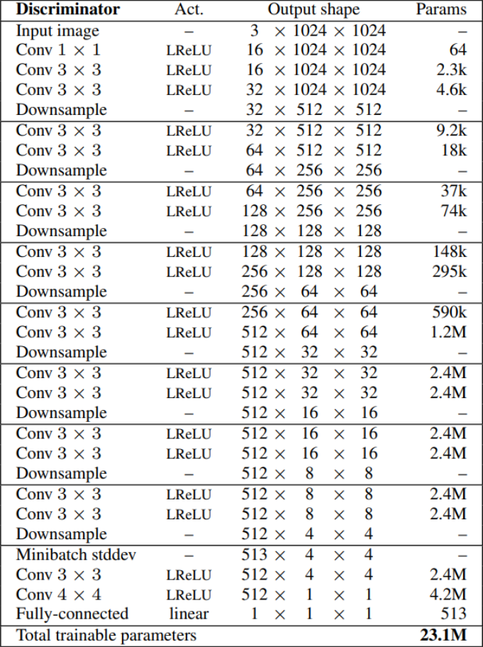
• Within the init half we ship in_channels and im_channels, and we initialize leaky by LeakyReLu with the slide of 0.2,  prog_blocks (keep in mind they’re going to be in reverse ordering, we downsample as an alternative of upsampling) by ModuleList() that can comprise all of the progressive blocks, rgb_blocks by ModuleList() that can comprise all of the RGB blocks, initial_rgb by WSConv2d that maps img_channels(3 for RGB) to in_channels, avg_pool for downsampling and remaining black which is the one totally different sample from others (see the determine above).
• Within the fade_in half, we ship alpha, downscaled from the typical pooling, out from the conv layer, and we return  [alpha * out + (1 – alpha) * downscaled]
• For Minibatch std on Discriminator, we add the minibatch_std half once we take the std for every instance (throughout all channels, and pixels) then we repeat it for a single channel and concatenate it with the picture. On this means, the discriminator will get details about the variation within the batch/picture.
• Within the ahead half, we ship x, the alpha worth, and steps, and it going to be precisely the other of the ahead half within the generator. Within the preliminary step, we convert the picture from RGB to in_channels relying on the picture dimension, we verify if steps=0 whether it is we simply use minibatch_std  and the ultimate block, in any other case, we fade_in between downscaled and out, then we run by means of the progressive block that corresponds to the decision of ‘out’, we downsample and we repeat that till we attain the decision that we would like relying on the steps, then we run it by means of minibatch_std and on the finish we return the final_block.

class Discriminator(nn.Module):
    def __init__(self, in_channels, img_channels=3):
        tremendous(Discriminator, self).__init__()
        self.prog_blocks, self.rgb_layers = nn.ModuleList([]), nn.ModuleList([])
        self.leaky = nn.LeakyReLU(0.2)

        # right here we work again methods from elements as a result of the discriminator
        # ought to be mirrored from the generator. So the primary prog_block and
        # rgb layer we append will work for enter dimension 1024x1024, then 512->256-> and so forth
        for i in vary(len(elements) - 1, 0, -1):
            conv_in = int(in_channels * elements[i])
            conv_out = int(in_channels * elements[i - 1])
            self.prog_blocks.append(ConvBlock(conv_in, conv_out, use_pixelnorm=False))
            self.rgb_layers.append(
                WSConv2d(img_channels, conv_in, kernel_size=1, stride=1, padding=0)
            )

        # maybe complicated identify "initial_rgb" that is simply the RGB layer for 4x4 enter dimension
        # did this to "mirror" the generator initial_rgb
        self.initial_rgb = WSConv2d(
            img_channels, in_channels, kernel_size=1, stride=1, padding=0
        )
        self.rgb_layers.append(self.initial_rgb)
        self.avg_pool = nn.AvgPool2d(
            kernel_size=2, stride=2
        )  # down sampling utilizing avg pool

        # that is the block for 4x4 enter dimension
        self.final_block = nn.Sequential(
            # +1 to in_channels as a result of we concatenate from MiniBatch std
            WSConv2d(in_channels + 1, in_channels, kernel_size=3, padding=1),
            nn.LeakyReLU(0.2),
            WSConv2d(in_channels, in_channels, kernel_size=4, padding=0, stride=1),
            nn.LeakyReLU(0.2),
            WSConv2d(
                in_channels, 1, kernel_size=1, padding=0, stride=1
            ),  # we use this as an alternative of linear layer
        )

    def fade_in(self, alpha, downscaled, out):
        """Used to fade in downscaled utilizing avg pooling and output from CNN"""
        # alpha ought to be scalar inside [0, 1], and upscale.form == generated.form
        return alpha * out + (1 - alpha) * downscaled

    def minibatch_std(self, x):
        batch_statistics = (
            torch.std(x, dim=0).imply().repeat(x.form[0], 1, x.form[2], x.form[3])
        )
        # we take the std for every instance (throughout all channels, and pixels) then we repeat it
        # for a single channel and concatenate it with the picture. On this means the discriminator
        # will get details about the variation within the batch/picture
        return torch.cat([x, batch_statistics], dim=1)

    def ahead(self, x, alpha, steps):
        # the place we must always begin within the record of prog_blocks, possibly a bit complicated however
        # the final is for the 4x4. So instance as an instance steps=1, then we must always begin
        # on the second to final as a result of input_size might be 8x8. If steps==0 we simply
        # use the ultimate block
        cur_step = len(self.prog_blocks) - steps

        # convert from rgb as preliminary step, it will rely on
        # the picture dimension (every can have it is on rgb layer)
        out = self.leaky(self.rgb_layers[cur_step](x))

        if steps == 0:  # i.e, picture is 4x4
            out = self.minibatch_std(out)
            return self.final_block(out).view(out.form[0], -1)

        # as a result of prog_blocks may change the channels, for down scale we use rgb_layer
        # from earlier/smaller dimension which in our case correlates to +1 within the indexing
        downscaled = self.leaky(self.rgb_layers[cur_step + 1](self.avg_pool(x)))
        out = self.avg_pool(self.prog_blocks[cur_step](out))

        # the fade_in is finished first between the downscaled and the enter
        # that is reverse from the generator
        out = self.fade_in(alpha, downscaled, out)

        for step in vary(cur_step + 1, len(self.prog_blocks)):
            out = self.prog_blocks[step](out)
            out = self.avg_pool(out)

        out = self.minibatch_std(out)
        return self.final_block(out).view(out.form[0], -1)

Utils

Within the code snippet beneath you’ll find the gradient_penalty perform for WGAN-GP loss.

def gradient_penalty(critic, actual, faux, alpha, train_step, gadget="cpu"):
    BATCH_SIZE, C, H, W = actual.form
    beta = torch.rand((BATCH_SIZE, 1, 1, 1)).repeat(1, C, H, W).to(gadget)
    interpolated_images = actual * beta + faux.detach() * (1 - beta)
    interpolated_images.requires_grad_(True)

    # Calculate critic scores
    mixed_scores = critic(interpolated_images, alpha, train_step)
 
    # Take the gradient of the scores with respect to the photographs
    gradient = torch.autograd.grad(
        inputs=interpolated_images,
        outputs=mixed_scores,
        grad_outputs=torch.ones_like(mixed_scores),
        create_graph=True,
        retain_graph=True,
    )[0]
    gradient = gradient.view(gradient.form[0], -1)
    gradient_norm = gradient.norm(2, dim=1)
    gradient_penalty = torch.imply((gradient_norm - 1) ** 2)
    return gradient_penalty

Within the code snippet beneath you’ll find the generate_examples perform that takes the generator gen, the variety of steps to establish the present decision, and a quantity n=100. The objective of this perform is to generate n faux photographs and save them because of this.

def generate_examples(gen, steps, n=100):

    gen.eval()
    alpha = 1.0
    for i in vary(n):
        with torch.no_grad():
            noise = torch.randn(1, Z_DIM, 1, 1).to(DEVICE)
            img = gen(noise, alpha, steps)
            if not os.path.exists(f'saved_examples/step{steps}'):
                os.makedirs(f'saved_examples/step{steps}')
            save_image(img*0.5+0.5, f"saved_examples/step{steps}/img_{i}.png")
    gen.prepare()

Coaching

On this part, we are going to prepare our ProGAN

First, let’s use this line of code to provide us some extra efficiency advantages.

torch.backends.cudnn.benchmarks = True

Prepare perform

First, we loop over all of the mini-batch sizes that we create with the DataLoader, and we take simply the photographs as a result of we do not want a label, then we establish the present batch dimension as a result of we’d like it later.

Then we arrange the coaching for the discriminatorCritic once we wish to maximize E(critic(actual)) – E(critic(faux)). This equation means how a lot the critic can distinguish between actual and faux photographs if we have now a big worth meaning the distinction between them is giant, if the worth is null meaning the critic cannot distinguish between them in any respect.

After that, we arrange the coaching for the generator once we wish to maximize E(critic(faux)). As a result of the generator desires to idiot the critic, so maximizing this equation means making this E(critic(actual)) – E(critic(faux)) a smaller worth, which is the other of what the critic need.

Lastly, we replace the alpha worth for fade_in and make sure that it’s between 0 and 1, and we return it.

def train_fn(
    critic,
    gen,
    loader,
    dataset,
    step,
    alpha,
    opt_critic,
    opt_gen,
):
    loop = tqdm(loader, depart=True)
    for batch_idx, (actual, _) in enumerate(loop):
        actual = actual.to(DEVICE)
        cur_batch_size = actual.form[0]

        # Prepare Critic: max E[critic(real)] - E[critic(fake)] <-> min -E[critic(real)] + E[critic(fake)]
        # which is equal to minimizing the adverse of the expression
        noise = torch.randn(cur_batch_size, Z_DIM, 1, 1).to(DEVICE)

        faux = gen(noise, alpha, step)
        critic_real = critic(actual, alpha, step)
        critic_fake = critic(faux.detach(), alpha, step)
        gp = gradient_penalty(critic, actual, faux, alpha, step, gadget=DEVICE)
        loss_critic = (
            -(torch.imply(critic_real) - torch.imply(critic_fake))
            + LAMBDA_GP * gp
            + (0.001 * torch.imply(critic_real ** 2))
        )

        critic.zero_grad()
        loss_critic.backward()
        opt_critic.step()

        # Prepare Generator: max E[critic(gen_fake)] <-> min -E[critic(gen_fake)]
        gen_fake = critic(faux, alpha, step)
        loss_gen = -torch.imply(gen_fake)

        gen.zero_grad()
        loss_gen.backward()
        opt_gen.step()

        # Replace alpha and guarantee lower than 1
        alpha += cur_batch_size / (
            (PROGRESSIVE_EPOCHS[step] * 0.5) * len(dataset)
        )
        alpha = min(alpha, 1)

        loop.set_postfix(
            gp=gp.merchandise(),
            loss_critic=loss_critic.merchandise(),
        )
        

    return alpha

Coaching

Now since we have now every thing let’s put them collectively to coach our ProGAN.

We begin by initializing the generator, the discriminator/critic, and optimizers in the identical means that they did within the paper, then convert the generator and the critic into prepare mode, then loop over PROGRESSIVE_EPOCHS, and in every loop, we prepare the mannequin variety of epoch instances, then we generate some faux photographs and save them, because of this, utilizing generate_examples perform, and at last, we progress to the subsequent picture decision.

# initialize gen and disc, notice: discriminator we referred to as critic,
# in response to WGAN paper (because it not outputs between [0, 1])
gen = Generator(
    Z_DIM, IN_CHANNELS, img_channels=CHANNELS_IMG
).to(DEVICE)
critic = Discriminator(
    IN_CHANNELS, img_channels=CHANNELS_IMG
).to(DEVICE)

# initialize optimizers
opt_gen = optim.Adam(gen.parameters(), lr=LEARNING_RATE, betas=(0.0, 0.99))
opt_critic = optim.Adam(
    critic.parameters(), lr=LEARNING_RATE, betas=(0.0, 0.99)
)


gen.prepare()
critic.prepare()

step = int(log2(START_TRAIN_AT_IMG_SIZE / 4))
for num_epochs in PROGRESSIVE_EPOCHS:
    alpha = 1e-5  # begin with very low alpha, you can begin with alpha=0
    loader, dataset = get_loader(4 * 2 ** step)  # 4->0, 8->1, 16->2, 32->3, 64 -> 4
    print(f"Present picture dimension: {4 * 2 ** step}")

    for epoch in vary(num_epochs):
        print(f"Epoch [{epoch+1}/{num_epochs}]")
        alpha = train_fn(
            critic,
            gen,
            loader,
            dataset,
            step,
            alpha,
            opt_critic,
            opt_gen,
        )
    generate_examples(gen, step, n=100)


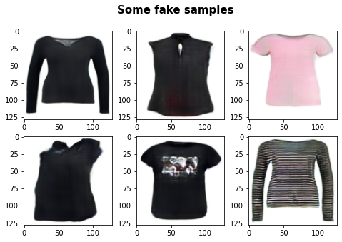
    step += 1  # progress to the subsequent img dimension

Consequence

Within the determine beneath you possibly can see the outcome that we receive after coaching this ProGAN on this dataset with 128*x 128 decision.

Conclusion

On this article, we make a clear, easy, and readable implementation from scratch of ProGAN with the important thing attributions from the paper (Progressive rising, Fading in new layers, Minibatch std on Discriminator, Normalization with PixelNorm, and Equalized Studying Fee) utilizing PyTorch.

Within the upcoming articles, we are going to clarify in depth and implement from scratch StyleGANs to generate additionally some cool trend.