

Convey this undertaking to life
This text is about StyleGAN2 from the paper Analyzing and Bettering the Picture High quality of StyleGAN, we’ll make a clear, easy, and readable implementation of it utilizing PyTorch, and attempt to replicate the unique paper as carefully as doable.
For those who did not learn the StyleGAN2 paper. or do not know the way it works and also you wish to perceive it, I extremely suggest you to take a look at this put up weblog the place I’m going throw the main points of it.
The dataset that we are going to use on this weblog is that this dataset from Kaggle which incorporates 16240 higher garments for ladies with 256*192 decision.
Load all dependencies we’d like
As at all times let’s begin by loading all dependencies we’d like.
We first will import torch since we’ll use PyTorch, and from there we import nn. That can assist us create and practice the networks, and likewise allow us to import optim, a package deal that implements numerous optimization algorithms (e.g. sgd, adam,..). From torchvision we import datasets and transforms to organize the info and apply some transforms.
We are going to import useful as F from torch.nn, DataLoader from torch.utils.information to create mini-batch sizes, save_image from torchvision.utils to avoid wasting pretend samples, log2 and sqrt kind math, Numpy for linear algebra, os for interplay with the working system, tqdm to point out progress bars, and at last matplotlib.pyplot to plot some pictures.
import torch
from torch import nn, optim
from torchvision import datasets, transforms
import torch.nn.useful as F
from torch.utils.information import DataLoader
from torchvision.utils import save_image
from math import log2, sqrt
import numpy as np
import os
from tqdm import tqdm
import matplotlib.pyplot as plt
Hyperparameters
- Initialize the DATASET by the trail of the true pictures.
- Initialize the machine by Cuda whether it is out there and CPU in any other case, the variety of epochs by 300, the training price by 0.001, and the batch measurement by 32.
- Initialize LOG_RESOLUTION by 7 as a result of we are attempting to generate 128*128 pictures, and a couple of^7 = 128. you possibly can change the worth relying on the decision of the pretend pictures that you really want.
- Within the unique paper, they initialize Z_DIM and W_DIM by 512, however I initialize them by 256 as an alternative for much less VRAM utilization and speed-up coaching. We may maybe even get higher outcomes if we doubled them.
- For StyleGAN2 we will use any of the GANs loss capabilities we wish, so I exploit WGAN-GP from the paper Improved Coaching of Wasserstein GANs. This loss incorporates a parameter identify λ and it’s normal to set λ = 10.
DATASET                 = "Girls garments"
DEVICE                  = "cuda" if torch.cuda.is_available() else "cpu"
EPOCHS                  = 300
LEARNING_RATE           = 1e-3
BATCH_SIZE              = 32
LOG_RESOLUTION          = 7 #for 128*128
Z_DIM                   = 256
W_DIM                   = 256
LAMBDA_GP               = 10
Get information loader
Now let’s create a perform get_loader to:
- Apply some transformation to the photographs (resize the photographs to the decision that we wish(2^LOG_RESOLUTION by 2^LOG_RESOLUTION), convert them to tensors, then apply some augmentation, and at last normalize them to be all of the pixels starting from -1 to 1).
- Put together the dataset by utilizing ImageFolder as a result of it is already structured in a pleasant means.
- Create mini-batch sizes utilizing DataLoader that take the dataset and batch measurement with shuffling the info.
- Lastly, return the loader.
def get_loader():
    remodel = transforms.Compose(
        [
            transforms.Resize((2 ** LOG_RESOLUTION, 2 ** LOG_RESOLUTION)),
            transforms.ToTensor(),
            transforms.RandomHorizontalFlip(p=0.5),
            transforms.Normalize(
                [0.5, 0.5, 0.5],
                [0.5, 0.5, 0.5],
            ),
        ]
    )
    dataset = datasets.ImageFolder(root=DATASET, remodel=remodel)
    loader = DataLoader(
        dataset,
        batch_size=BATCH_SIZE,
        shuffle=True,
    )
    return loader
Fashions implementation
Now let’s Implement the StyleGAN2 networks with the important thing attributions from the paper. We are going to attempt to make the implementation compact but additionally maintain it readable and comprehensible. Particularly, the important thing factors:
- Noise Mapping Community
- Weight demodulation (As an alternative of Adaptive Occasion Normalization (AdaIN))
- Skip connections (As an alternative of progressive rising)
- Perceptual path size normalization
Noise Mapping Community
Let’s create the MappingNetwork class which can be inherited from nn.Module.
- Within the init half we ship z_dim and w_din, and we outline the community mapping containing eight of EqualizedLinear, a category that we are going to implement later that equalizes the training price, and ReLu as an activation perform
- Within the ahead half, we initialize z_dim utilizing pixel norm then we return the community mapping.
class MappingNetwork(nn.Module):
    def __init__(self, z_dim, w_dim):
        tremendous().__init__()
        self.mapping = nn.Sequential(
            EqualizedLinear(z_dim, w_dim),
            nn.ReLU(),
            EqualizedLinear(z_dim, w_dim),
            nn.ReLU(),
            EqualizedLinear(z_dim, w_dim),
            nn.ReLU(),
            EqualizedLinear(z_dim, w_dim),
            nn.ReLU(),
            EqualizedLinear(z_dim, w_dim),
            nn.ReLU(),
            EqualizedLinear(z_dim, w_dim),
            nn.ReLU(),
            EqualizedLinear(z_dim, w_dim),
            nn.ReLU(),
            EqualizedLinear(z_dim, w_dim)
        )

    def ahead(self, x):
    	  x = x / torch.sqrt(torch.imply(x ** 2, dim=1, keepdim=True) + 1e-8)  # for PixelNorm
        return self.mapping(x)
Generator
Within the determine under you possibly can see the generator structure the place it begins with an preliminary fixed. Then it has a collection of blocks. The characteristic map decision is doubled at every block. Every block outputs an RGB picture and they’re scaled up and summed to get the ultimate RGB picture.
toRGB additionally has a mode modulation which isn’t proven within the determine to maintain it easy.
To make the code as clear as doable, within the implementation of the generator we’ll use three lessons that we are going to outline later (StyleBlock, toRGB, and GeneratorBlock).
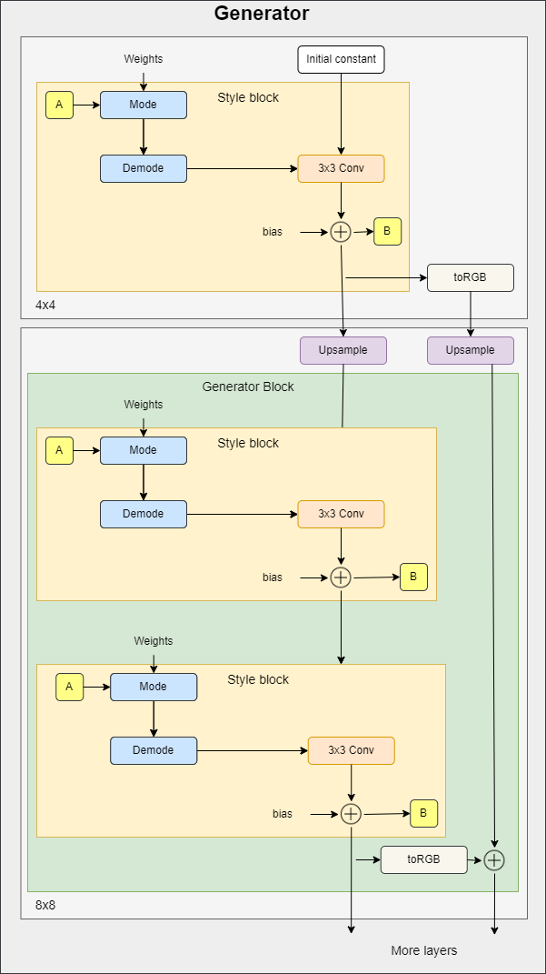
- Within the init half, we ship log_resolution which is the log2 of picture decision, W_DIM which s the dimensionality of w, n_featurese which is the variety of options within the convolution layer on the highest decision (ultimate block), max_features which is the utmost variety of options in any generator block. We calculate the variety of options for every block, we get the variety of generator blocks, and we initialize the trainable 4×4 fixed, the primary type block for 4×4 decision, the layer to get RGB, and the generator blocks.
- Within the ahead half, we ship in w for every generator block it has form [n_blocks, batch_size, W-dim], and input_noise which is the noise for every block, it is a record of pairs of noise tensors as a result of every block (besides the preliminary) has two noise inputs after every convolution layer (see the determine above). We get the batch measurement, increase the discovered fixed to match the batch measurement, run it into the primary type block, get the RGB picture, then run it once more into the remainder of the generator blocks after upsampling. Lastly, return the final RGB picture with tanh as an activation perform. The rationale why we use tanh is that would be the output(the generated picture) and we wish the pixels to vary between 1 and -1.
class Generator(nn.Module):

    def __init__(self, log_resolution, W_DIM, n_features = 32, max_features = 256):

        tremendous().__init__()

        options = [min(max_features, n_features * (2 ** i)) for i in range(log_resolution - 2, -1, -1)]
        self.n_blocks = len(options)

        self.initial_constant = nn.Parameter(torch.randn((1, options[0], 4, 4)))

        self.style_block = StyleBlock(W_DIM, options[0], options[0])
        self.to_rgb = ToRGB(W_DIM, options[0])

        blocks = [GeneratorBlock(W_DIM, features[i - 1], options[i]) for i in vary(1, self.n_blocks)]
        self.blocks = nn.ModuleList(blocks)

    def ahead(self, w, input_noise):

        batch_size = w.form[1]

        x = self.initial_constant.increase(batch_size, -1, -1, -1)
        x = self.style_block(x, w[0], input_noise[0][1])
        rgb = self.to_rgb(x, w[0])

        for i in vary(1, self.n_blocks):
            x = F.interpolate(x, scale_factor=2, mode="bilinear")
            x, rgb_new = self.blocks[i - 1](x, w[i], input_noise[i])
            rgb = F.interpolate(rgb, scale_factor=2, mode="bilinear") + rgb_new

        return torch.tanh(rgb)
Generator Block
Within the determine under you possibly can see the generator block structure which consists of two type blocks (3×3 convolutions with type modulation) and RGB output.
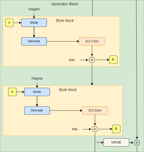
- Within the init half, we ship in W_DIM which is the dimensionality of w, in_features which is the variety of options within the enter characteristic map, and out_features which is the variety of options within the output characteristic map, then we initialize two type blocks and toRGB layer.
- Within the ahead half, we ship in x which is the enter characteristic map of the form [batch_size, in_features, height, width], w with the form [batch_size, W_DIM], and noise which is a tuple of two noise tensors of form [batch_size, 1, height, width], then we run x into the 2 type blocks and we get the RGB picture utilizing the layer toRGB. Lastly, we return x and the RGB picture.
class GeneratorBlock(nn.Module):

    def __init__(self, W_DIM, in_features, out_features):

        tremendous().__init__()

        self.style_block1 = StyleBlock(W_DIM, in_features, out_features)
        self.style_block2 = StyleBlock(W_DIM, out_features, out_features)

        self.to_rgb = ToRGB(W_DIM, out_features)

    def ahead(self, x, w, noise):

        x = self.style_block1(x, w, noise[0])
        x = self.style_block2(x, w, noise[1])

        rgb = self.to_rgb(x, w)

        return x, rgb
Type Block
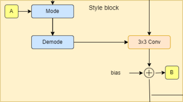
- Within the init half, we ship W_DIM, in_features, and out_features, then we initialize to_style by the type vector that we get from w (denoted by A within the diagram) with an equalized studying price linear layer (EqualizedLinear) that we are going to implement later, weight modulated convolution layer, noise scale, bias, and activation perform.
- Within the ahead half, we ship x, w, and noise, then we get the type vector s, run x and s into the load modulated convolution, scale and add noise, and at last add bias and consider the activation perform.
class StyleBlock(nn.Module):

    def __init__(self, W_DIM, in_features, out_features):

        tremendous().__init__()

        self.to_style = EqualizedLinear(W_DIM, in_features, bias=1.0)
        self.conv = Conv2dWeightModulate(in_features, out_features, kernel_size=3)
        self.scale_noise = nn.Parameter(torch.zeros(1))
        self.bias = nn.Parameter(torch.zeros(out_features))

        self.activation = nn.LeakyReLU(0.2, True)

    def ahead(self, x, w, noise):

        s = self.to_style(w)
        x = self.conv(x, s)
        if noise will not be None:
            x = x + self.scale_noise[None, :, None, None] * noise
        return self.activation(x + self.bias[None, :, None, None])
To RGB
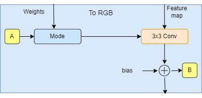
- Within the init half, we ship W_DIM, and options, then we initialize to_style by the type vector that we get from w (denoted by A within the diagram), weight modulated convolution layer, bias, and activation perform.
- Within the ahead half, we ship x, and w, then we get the type vector type, we run x and elegance into the load modulated convolution, and at last, we add bias and consider the activation perform.
class ToRGB(nn.Module):

    def __init__(self, W_DIM, options):

        tremendous().__init__()
        self.to_style = EqualizedLinear(W_DIM, options, bias=1.0)

        self.conv = Conv2dWeightModulate(options, 3, kernel_size=1, demodulate=False)
        self.bias = nn.Parameter(torch.zeros(3))
        self.activation = nn.LeakyReLU(0.2, True)

    def ahead(self, x, w):

        type = self.to_style(w)
        x = self.conv(x, type)
        return self.activation(x + self.bias[None, :, None, None])
Convolution with Weight Modulation and Demodulation
Convey this undertaking to life
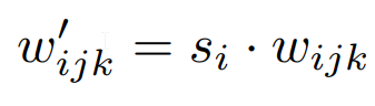
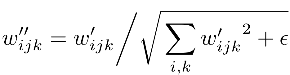
This class scales the convolution weights by the type vector and demodulates it by normalizing it.
- Within the init half, we ship in_features, out_features, kernel_size, demodulates which is a flag whether or not to normalize weights by its customary deviation, and eps which is the ϵ for normalizing, then we initialize the variety of output options, demodulate, padding measurement, Weights parameter with equalized studying price utilizing the category EqualizedWeight that we are going to implement later, and eps.
- Within the ahead half, we ship in x which is the enter characteristic map, and s which is a style-based scaling tensor, then we get the batch measurement, peak, and width from x, reshape the scales, get the training price equalized weights, then modulate x and s, and demodulate them if demodulates is True utilizing the equations under the place i is the enter channel, j is the output channel, and okay is the kernel index. And at last, we return x.
class Conv2dWeightModulate(nn.Module):

    def __init__(self, in_features, out_features, kernel_size,
                 demodulate = True, eps = 1e-8):

        tremendous().__init__()
        self.out_features = out_features
        self.demodulate = demodulate
        self.padding = (kernel_size - 1) // 2

        self.weight = EqualizedWeight([out_features, in_features, kernel_size, kernel_size])
        self.eps = eps

    def ahead(self, x, s):

        b, _, h, w = x.form

        s = s[:, None, :, None, None]
        weights = self.weight()[None, :, :, :, :]
        weights = weights * s

        if self.demodulate:
            sigma_inv = torch.rsqrt((weights ** 2).sum(dim=(2, 3, 4), keepdim=True) + self.eps)
            weights = weights * sigma_inv

        x = x.reshape(1, -1, h, w)

        _, _, *ws = weights.form
        weights = weights.reshape(b * self.out_features, *ws)

        x = F.conv2d(x, weights, padding=self.padding, teams=b)

        return x.reshape(-1, self.out_features, h, w)
Discriminator
Within the determine under you possibly can see the discriminator structure. It first transforms the picture with the decision 2LOG_RESOLUTION by 2LOG_RESOLUTION to a characteristic map of the identical decision after which runs it by way of a collection of blocks with residual connections. The decision is down-sampled by 2× at every block whereas doubling the variety of options.
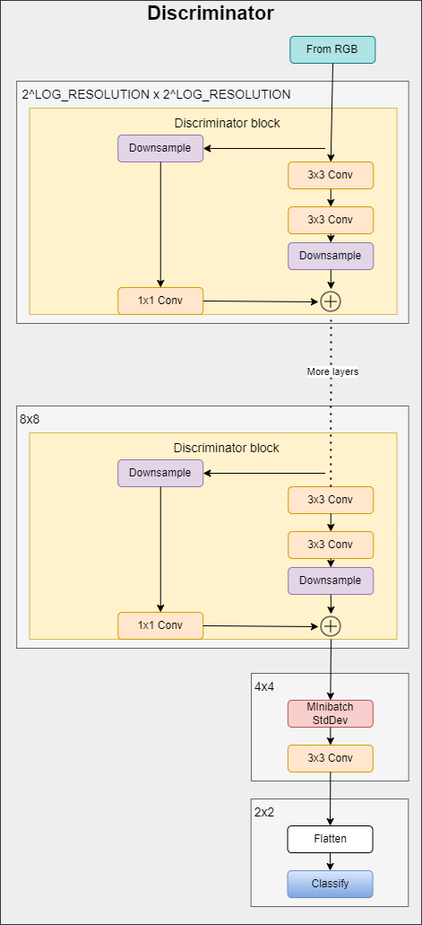
- Within the init half, we ship in log_resolution, n_feautures, and max_features, calculate the variety of options for every block, then initialize a layer with the identify from_rgb to transform the RGB picture to a characteristic map with n_features variety of options, variety of discriminator blocks, discriminator blocks, variety of options after including the map of the usual deviation, ultimate 3×3 convolution layer, and ultimate linear layer to get the classification.
- For Minibatch std on Discriminator, we add the minibatch_std half after we take the std for every instance (throughout all channels, and pixels) then we repeat it for a single channel and concatenate it with the picture. On this means, the discriminator will get details about the variation within the batch/picture.
- Within the ahead half, we ship in x which is the enter picture of the form [batch_size, 3, height, width], and we run it throw the from_RGB layer, discriminator blocks, minibatch_std, 3×3 convolution, flatten, and classification rating.
class Discriminator(nn.Module):

    def __init__(self, log_resolution, n_features = 64, max_features = 256):

        tremendous().__init__()

        options = [min(max_features, n_features * (2 ** i)) for i in range(log_resolution - 1)]

        self.from_rgb = nn.Sequential(
            EqualizedConv2d(3, n_features, 1),
            nn.LeakyReLU(0.2, True),
        )
        n_blocks = len(options) - 1
        blocks = [DiscriminatorBlock(features[i], options[i + 1]) for i in vary(n_blocks)]
        self.blocks = nn.Sequential(*blocks)

        final_features = options[-1] + 1
        self.conv = EqualizedConv2d(final_features, final_features, 3)
        self.ultimate = EqualizedLinear(2 * 2 * final_features, 1)

    def minibatch_std(self, x):
        batch_statistics = (
            torch.std(x, dim=0).imply().repeat(x.form[0], 1, x.form[2], x.form[3])
        )
        return torch.cat([x, batch_statistics], dim=1)

    def ahead(self, x):

        x = self.from_rgb(x)
        x = self.blocks(x)

        x = self.minibatch_std(x)
        x = self.conv(x)
        x = x.reshape(x.form[0], -1)
        return self.ultimate(x)
Discriminator Block
Within the determine under you possibly can see the discriminator block structure that consists of two 3×3 convolutions with a residual connection.
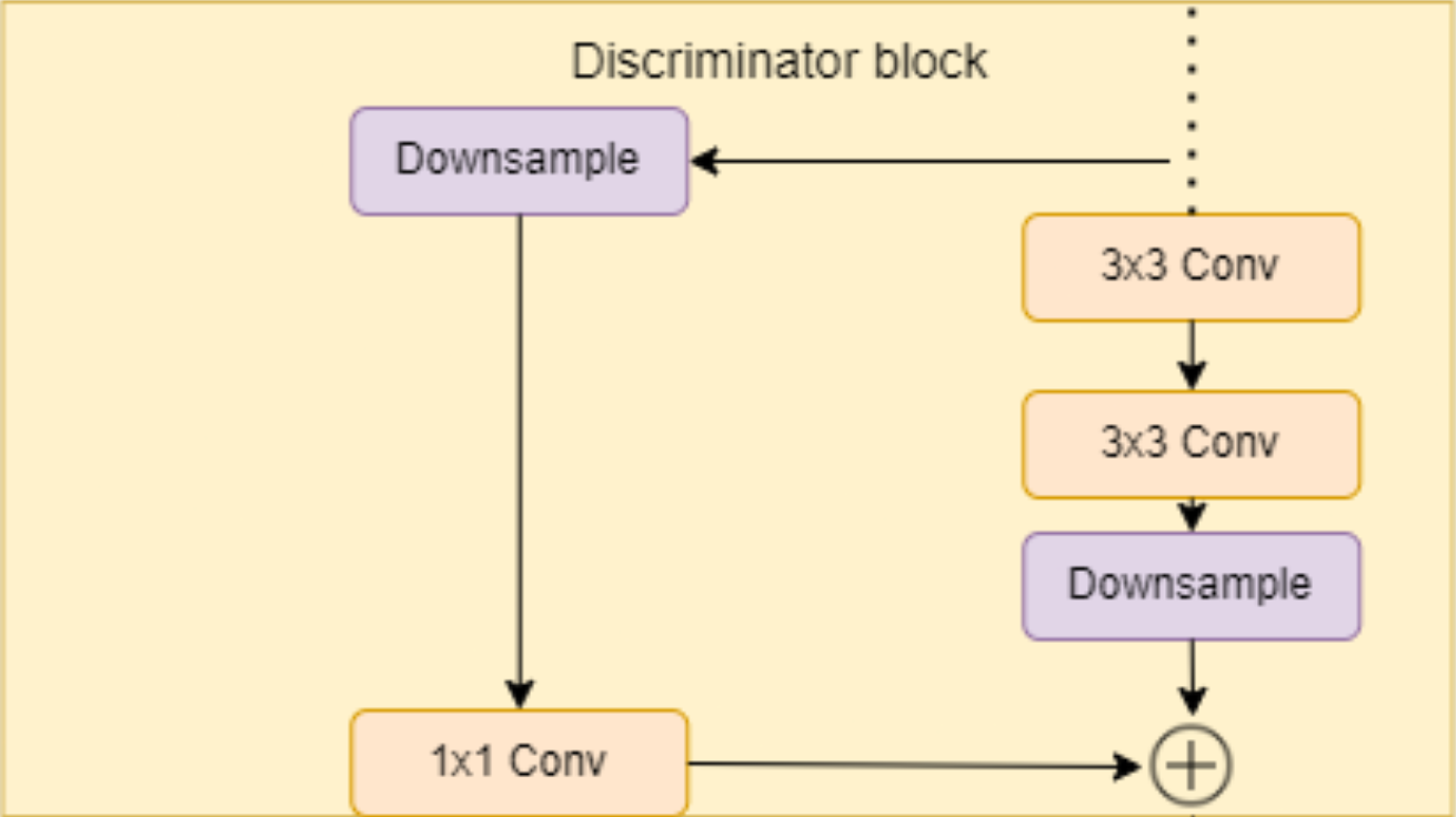
- Within the init half, we ship in in_features and out_features, and we initialize the residual block that incorporates down-sampling and a 1×1 convolution layer for the residual connection, the block layer that incorporates two 3×3 convolutions with Leaky Rely as activation perform, down_sample layer utilizing AvgPool2d, and the size issue that we are going to use after including the residual.
- Within the ahead half, we ship in x and we run it throw the residual connection to get a variable with the identify residual, then we run x throw the convolutions and downsample, then we add the residual and scale, and we return it.
class DiscriminatorBlock(nn.Module):

    def __init__(self, in_features, out_features):
        tremendous().__init__()
        self.residual = nn.Sequential(nn.AvgPool2d(kernel_size=2, stride=2), # down sampling utilizing avg pool
                                      EqualizedConv2d(in_features, out_features, kernel_size=1))

        self.block = nn.Sequential(
            EqualizedConv2d(in_features, in_features, kernel_size=3, padding=1),
            nn.LeakyReLU(0.2, True),
            EqualizedConv2d(in_features, out_features, kernel_size=3, padding=1),
            nn.LeakyReLU(0.2, True),
        )

        self.down_sample = nn.AvgPool2d(
            kernel_size=2, stride=2
        )  # down sampling utilizing avg pool

        self.scale = 1 / sqrt(2)

    def ahead(self, x):
        residual = self.residual(x)

        x = self.block(x)
        x = self.down_sample(x)

        return (x + residual) * self.scale
Studying-rate Equalized Linear Layer
Now it’s time to implement EqualizedLinear that we use earlier in virtually each class to equalize the training price for a linear layer.
- Within the init half, we ship in in_features, out_features, and bias. We initialize the load by a category EqualizedWeight that we are going to outline later, and we initialize the bias.
- Within the ahead half, we ship in x and return the linear transformation of x, weight, and bias
class EqualizedLinear(nn.Module):

    def __init__(self, in_features, out_features, bias = 0.):

        tremendous().__init__()
        self.weight = EqualizedWeight([out_features, in_features])
        self.bias = nn.Parameter(torch.ones(out_features) * bias)

    def ahead(self, x: torch.Tensor):
        return F.linear(x, self.weight(), bias=self.bias)
Studying-rate Equalized 2D Convolution Layer
Now let’s implement EqualizedConv2d that we use earlier to equalize the training price for a convolution layer.
- Within the init half, we ship in in_features, out_features, kernel_size, and padding. We initialize the padding, the load by a category EqualizedWeight that we are going to outline later, and the bias.
- Within the ahead half, we ship in x and return the convolution of x, weight, bias, and padding.
class EqualizedConv2d(nn.Module):

    def __init__(self, in_features, out_features,
                 kernel_size, padding = 0):

        tremendous().__init__()
        self.padding = padding
        self.weight = EqualizedWeight([out_features, in_features, kernel_size, kernel_size])
        self.bias = nn.Parameter(torch.ones(out_features))

    def ahead(self, x: torch.Tensor):
        return F.conv2d(x, self.weight(), bias=self.bias, padding=self.padding)
Studying-rate Equalized Weights Parameter
Now let’s implement EqualizedWeight class that we use in Studying-rate Equalized Linear Layer and Studying-rate Equalized 2D Convolution Layer.
That is based mostly on equalized studying price launched within the ProGAN paper. As an alternative of initializing weights at N(0,c) they initialize weights to N(0,1) after which multiply them by c when utilizing it.
- Within the init half, we ship within the form of the load parameter, we initialize the fixed c and the weights with N(0,1).
- Within the ahead half, we multiply weights by c and return.
class EqualizedWeight(nn.Module):

    def __init__(self, form):

        tremendous().__init__()

        self.c = 1 / sqrt(np.prod(form[1:]))
        self.weight = nn.Parameter(torch.randn(form))

    def ahead(self):
        return self.weight * self.c
Perceptual path size normalization
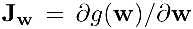
Perceptual path size normalization encourages a fixed-size step in w to lead to a fixed-magnitude change within the picture.
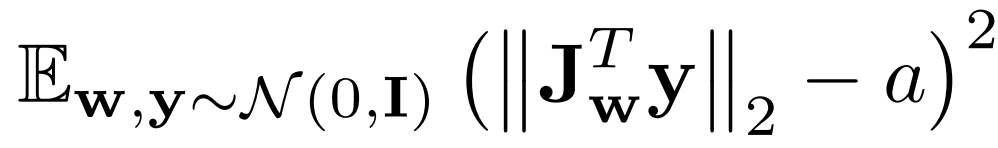
The place Jw is calculated with the equation under, w is sampled from the mapping community, y are pictures with noise N(0, I), and a is the exponential shifting common because the coaching progresses.
- Within the init half, we ship in beta which is the fixed β used to calculate the exponential shifting common a. Initialize beta, steps by the number of steps calculated N, exp_sum_a by the exponential sum of JwTy.
- Within the ahead half, we ship in x which is the batch of w of form [batch_size, W_DIM] and x are the generated pictures of form [batch_size, 3, height, width], get the machine and variety of pixels, calculate the equations above, replace exponential sum, increment N, and return the penalty.
class PathLengthPenalty(nn.Module):

    def __init__(self, beta):

        tremendous().__init__()

        self.beta = beta
        self.steps = nn.Parameter(torch.tensor(0.), requires_grad=False)

        self.exp_sum_a = nn.Parameter(torch.tensor(0.), requires_grad=False)

    def ahead(self, w, x):

        machine = x.machine
        image_size = x.form[2] * x.form[3]
        y = torch.randn(x.form, machine=machine)

        output = (x * y).sum() / sqrt(image_size)
        sqrt(image_size)

        gradients, *_ = torch.autograd.grad(outputs=output,
                                            inputs=w,
                                            grad_outputs=torch.ones(output.form, machine=machine),
                                            create_graph=True)

        norm = (gradients ** 2).sum(dim=2).imply(dim=1).sqrt()

        if self.steps > 0:

            a = self.exp_sum_a / (1 - self.beta ** self.steps)

            loss = torch.imply((norm - a) ** 2)
        else:
            loss = norm.new_tensor(0)

        imply = norm.imply().detach()
        self.exp_sum_a.mul_(self.beta).add_(imply, alpha=1 - self.beta)
        self.steps.add_(1.)

        return loss
Utils
gradient_penalty
Within the code snippet under you will discover the gradient_penalty perform for WGAN-GP loss.
def gradient_penalty(critic, actual, pretend,machine="cpu"):
    BATCH_SIZE, C, H, W = actual.form
    beta = torch.rand((BATCH_SIZE, 1, 1, 1)).repeat(1, C, H, W).to(machine)
    interpolated_images = actual * beta + pretend.detach() * (1 - beta)
    interpolated_images.requires_grad_(True)

    # Calculate critic scores
    mixed_scores = critic(interpolated_images)

    # Take the gradient of the scores with respect to the photographs
    gradient = torch.autograd.grad(
        inputs=interpolated_images,
        outputs=mixed_scores,
        grad_outputs=torch.ones_like(mixed_scores),
        create_graph=True,
        retain_graph=True,
    )[0]
    gradient = gradient.view(gradient.form[0], -1)
    gradient_norm = gradient.norm(2, dim=1)
    gradient_penalty = torch.imply((gradient_norm - 1) ** 2)
    return gradient_penalty
Pattern W
This perform samples Z randomly and will get W from the mapping community.
def get_w(batch_size):

    z = torch.randn(batch_size, W_DIM).to(DEVICE)
    w = mapping_network(z)
    return w[None, :, :].increase(LOG_RESOLUTION, -1, -1)
Generate noise
This perform generates noise for every generator block
def get_noise(batch_size):

        noise = []
        decision = 4

        for i in vary(LOG_RESOLUTION):
            if i == 0:
                n1 = None
            else:
                n1 = torch.randn(batch_size, 1, decision, decision, machine=DEVICE)
            n2 = torch.randn(batch_size, 1, decision, decision, machine=DEVICE)

            noise.append((n1, n2))

            decision *= 2

        return noise
Within the code snippet under you will discover the generate_examples perform that takes the generator gen, the variety of epochs, and a quantity n=100. The aim of this perform is to generate n pretend pictures and save them consequently for every epoch.
def generate_examples(gen, epoch, n=100):

    gen.eval()
    alpha = 1.0
    for i in vary(n):
        with torch.no_grad():
            w     = get_w(1)
            noise = get_noise(1)
            img = gen(w, noise)
            if not os.path.exists(f'saved_examples/epoch{epoch}'):
                os.makedirs(f'saved_examples/epoch{epoch}')
            save_image(img*0.5+0.5, f"saved_examples/epoch{epoch}/img_{i}.png")

    gen.practice()
Coaching
On this part, we’ll practice our StyleGAN2.
Let’s begin by creating the practice perform that takes the discriminator/critic, gen for generator, path_length_penalty that we are going to use each 16 epochs, loader, and the optimizers for the networks. We begin by looping over all of the mini-batch sizes that we create with the DataLoader, and we take simply the photographs as a result of we do not want a label.
Then we arrange the coaching for the discriminatorCritic after we wish to maximize E(critic(actual)) – E(critic(pretend)). This equation means how a lot the critic can distinguish between actual and pretend pictures.
After that, we arrange the coaching for the generator and mapping community after we wish to maximize E(critic(pretend)), and we add to this perform a perceptual path size each 16 epochs.
Lastly, we replace the loop.
def train_fn(
    critic,
    gen,
    path_length_penalty,
    loader,
    opt_critic,
    opt_gen,
    opt_mapping_network,
):
    loop = tqdm(loader, go away=True)

    for batch_idx, (actual, _) in enumerate(loop):
        actual = actual.to(DEVICE)
        cur_batch_size = actual.form[0]

        w     = get_w(cur_batch_size)
        noise = get_noise(cur_batch_size)
        with torch.cuda.amp.autocast():
            pretend = gen(w, noise)
            critic_fake = critic(pretend.detach())

            critic_real = critic(actual)
            gp = gradient_penalty(critic, actual, pretend, machine=DEVICE)
            loss_critic = (
                -(torch.imply(critic_real) - torch.imply(critic_fake))
                + LAMBDA_GP * gp
                + (0.001 * torch.imply(critic_real ** 2))
            )

        critic.zero_grad()
        loss_critic.backward()
        opt_critic.step()

        gen_fake = critic(pretend)
        loss_gen = -torch.imply(gen_fake)

        if batch_idx % 16 == 0:
            plp = path_length_penalty(w, pretend)
            if not torch.isnan(plp):
                loss_gen = loss_gen + plp

        mapping_network.zero_grad()
        gen.zero_grad()
        loss_gen.backward()
        opt_gen.step()
        opt_mapping_network.step()

        loop.set_postfix(
            gp=gp.merchandise(),
            loss_critic=loss_critic.merchandise(),
        )
Now let’s initialize the loader, the networks, and the optimizers, and make the networks within the coaching mode
loader              = get_loader()

gen                 = Generator(LOG_RESOLUTION, W_DIM).to(DEVICE)
critic              = Discriminator(LOG_RESOLUTION).to(DEVICE)
mapping_network     = MappingNetwork(Z_DIM, W_DIM).to(DEVICE)
path_length_penalty = PathLengthPenalty(0.99).to(DEVICE)

opt_gen             = optim.Adam(gen.parameters(), lr=LEARNING_RATE, betas=(0.0, 0.99))
opt_critic          = optim.Adam(critic.parameters(), lr=LEARNING_RATE, betas=(0.0, 0.99))
opt_mapping_network = optim.Adam(mapping_network.parameters(), lr=LEARNING_RATE, betas=(0.0, 0.99))

gen.practice()
critic.practice()
mapping_network.practice()
Now let’s practice the networks utilizing the coaching loop, and avoid wasting pretend samples in every 50 epoch.
loader = get_loader()

for epoch in vary(EPOCHS):
    train_fn(
        critic,
        gen,
        path_length_penalty,
        loader,
        opt_critic,
        opt_gen,
        opt_mapping_network,
    )
    if epoch % 50 == 0:
    	generate_examples(gen, epoch)
Conclusion
On this article, we make a clear, easy, and readable implementation from scratch for an enormous undertaking which is StyleGAN2 utilizing PyTorch. we attempt to replicate the unique paper as carefully as doable.