
It is common information that in a convolutional neural community, the processes of convolution and pooling work collectively to be able to archive a ultimate mannequin goal. Nevertheless, there are some fairly useful bye-products of those two processes that are important to the way in which convolutional neural networks course of photos; they’re referred to as translation invariance and translation equivariance.
#  article dependencies
import torch
import torch.nn as nn
import torch.nn.practical as F
import torchvision
import numpy as np
import matplotlib.pyplot as plt
import cv2
from tqdm.pocket book import tqdm
import seaborn as sns
from torchvision.utils import make_grid
Translation in a Laptop Imaginative and prescient Context
In a language context translation means interpretation of textual content or speech from one language to the opposite. Nevertheless, in physics, translation (as in translational movement) merely means the motion of a physique from one location to a different on a spatial airplane.
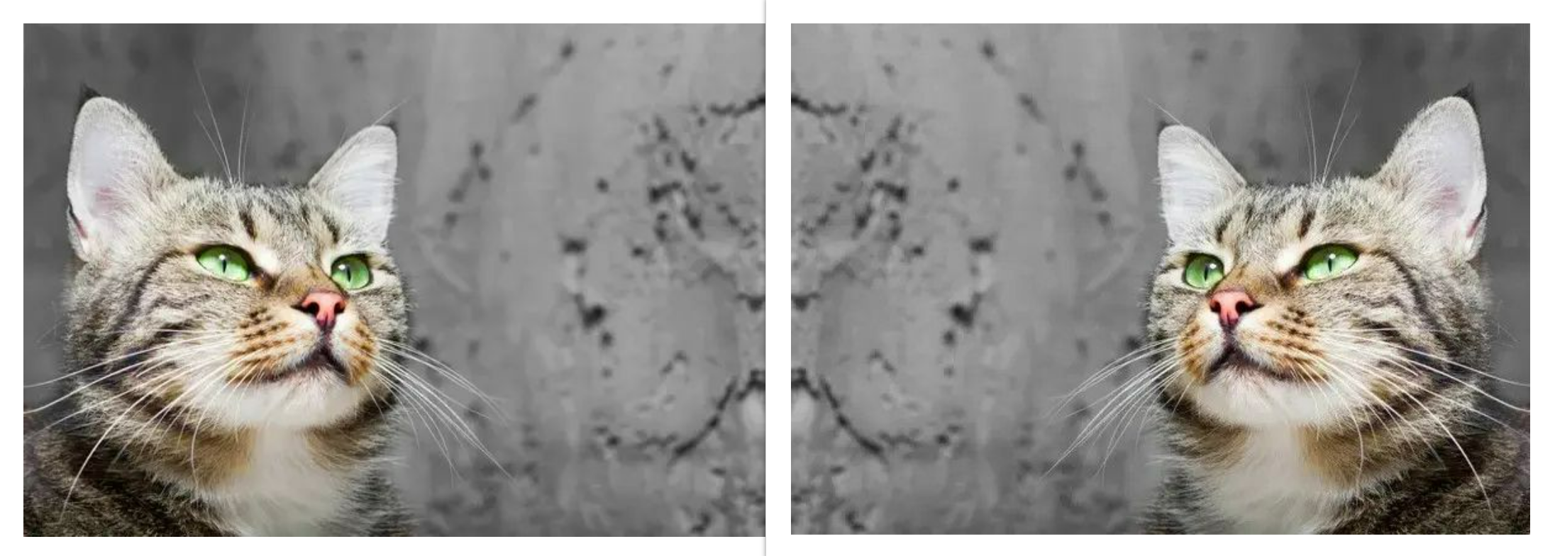
Translation in a pc imaginative and prescient context is extra much like the physics definition as translation of an object in a picture implies the motion of that object from one location within the picture to a different. Take into account the picture beneath, the yellow pixel at index [2, 2] on the left is moved to index [7, 7], it may be mentioned that the pixel has undergone translation from the highest left nook to the underside proper nook.
Why It Issues
Utilizing the pictures above as some extent of reference, if the yellow pixel had been to be shifted by only one pixel to the proper (to index [2, 3]) a human would nonetheless most likely see these photos as basically the identical. Nevertheless to a pc the 2 photos will now be fully totally different; so from a pc imaginative and prescient standpoint it’s crucial to understand how a convolutional neural community treats these two photos based mostly on translation of objects current within the picture.
Translation Equivariance
Equivariance in a mathematical context refers to a situation the place a operate offers the identical output albeit with a unique order when the order of the enter upon which it acts on adjustments. Talking contextually as regards to convolutional neural networks, translation equivariance implies that even when the place of an object in a picture is modified the identical options might be detected even at it is new place.
As you might need guessed, convolution layers might be answerable for this conduct as they’re tasked with the burden of function extraction. To analyze this, take into account the picture beneath, it’s fabricated from two distinct photos with one being the mirrored model of the opposite. Utilizing these photos we are going to make the most of the customized written convolution operate, as outlined within the code block beneath, in extracting options/detecting edges within the picture.
def convolve(image_path, filter, title=""):
    """This operate performs convolution over a picture
    with the goal of edge detection"""

    if kind(image_path) == np.ndarray:
      picture = image_path
    else:
      #  studying picture
      picture = cv2.imread(image_path, cv2.IMREAD_GRAYSCALE)

    #  defining filter measurement
    filter_size = filter.form[0]

    #  creating an array to retailer convolutions
    convolved = np.zeros(((picture.form[0] - filter_size) + 1,
                      (picture.form[1] - filter_size) + 1))

    #  performing convolution
    for i in tqdm(vary(picture.form[0])):
      for j in vary(picture.form[1]):
        attempt:
          convolved[i,j] = (picture[i:(i+filter_size),
                                  j:(j+filter_size)] * filter).sum()
        besides Exception:
          move

    #  changing to tensor
    convolved = torch.tensor(convolved)
    #  making use of relu activation
    convolved = F.relu(convolved)

    #  producing plots
    determine, axes = plt.subplots(1,2, dpi=120)
    plt.suptitle(title)
    axes[0].imshow(picture, cmap='grey')
    axes[0].axis('off')
    axes[0].set_title('authentic')
    axes[1].imshow(convolved,)
    axes[1].axis('off')
    axes[1].set_title('convolved')
    return convolved
Utilizing the above outlined operate, we might be detecting vertical edges in each photos utilizing the Sobel vertical edge detection filter outlined beneath.
#  defining sobel filter
sobel_y = np.array(([-1,0,1],
                    [-1,0,1],
                    [-1,0,1]))

#  detecting edges in picture
convolve('picture.jpg', filter=sobel_y)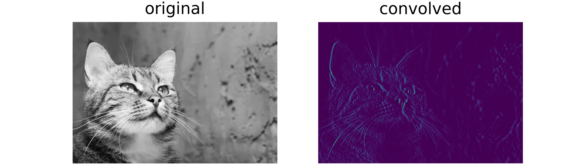
#  detecting edge in mirrored model of picture
convolve('image_mirrored.jpg', filter=sobel_y)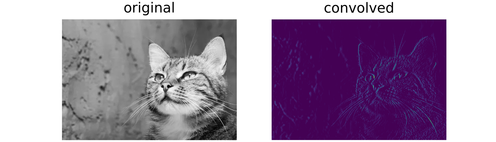
From the outcomes obtained above, it’s clear that though the place of the article of curiosity within the picture had modified, the identical edges had been detected. This provides credence to the truth that convolutional neural networks, by advantage of their convolution layers, are the truth is translation equivariant.
Translation Invariance
Translation invariance refers to a scenario the place a change in place of an object doesn’t have an effect on the character of the output. Though they may sound contrasting, translation invariance and translation equivariance aren’t essentially mutually unique, they’ll each happen on the similar time though beneath totally different contexts as we are going to see beneath.
Not like translation equivariance which is led to by convolution operations in CNNs, translation invariance is a spinoff of the pooling course of. The entire thought is that even when an object of curiosity is moved round in a picture, pooling brings the article into focus in order that finally their most salient options (pixels) find yourself in the identical approximate location. To analyze this, take into account the max pooling operate written beneath, utilizing this operate we can generate max pooled representations from photos of curiosity.
def max_pool(picture, kernel_size=2, visualize=False, title=""):
      """
      This operate replicates the maxpooling
      course of
      """

      #  assessing picture parameter
      if kind(picture) is np.ndarray and len(picture.form)==2:
        picture = picture
      else:
        picture = cv2.imread(picture, cv2.IMREAD_GRAYSCALE)

      #  creating an empty listing to retailer pooling
      pooled = np.zeros((picture.form[0]//kernel_size,
                        picture.form[1]//kernel_size))

      #  instantiating counter
      ok=-1
      #  maxpooling
      for i in tqdm(vary(0, picture.form[0], kernel_size)):
        ok+=1
        l=-1
        if ok==pooled.form[0]:
          break
        for j in vary(0, picture.form[1], kernel_size):
          l+=1
          if l==pooled.form[1]:
            break
          attempt:
            pooled[k,l] = (picture[i:(i+kernel_size),
                                j:(j+kernel_size)]).max()
          besides ValueError:
            move

      if visualize:
        #  displaying outcomes
        determine, axes = plt.subplots(1,2, dpi=120)
        plt.suptitle(title)
        axes[0].imshow(picture, cmap='grey')
        axes[0].set_title('reference picture')
        axes[1].imshow(pooled, cmap='grey')
        axes[1].set_title('averagepooled')
      return pooled
The operate beneath helps to iteratively apply the max pooling operate on a picture and return a visualization of each the reference picture and it is max pooled representations.
def visualize_pooling(picture, iterations, kernel=2, dpi=700):
      """
      This operate helps to visualise a number of
      iterations of the pooling course of
      """
      #picture = cv2.imread(picture, cv2.IMREAD_GRAYSCALE)

      #  creating empty listing to carry swimming pools
      swimming pools = []
      swimming pools.append(picture)

      #  performing pooling
      for iteration in vary(iterations):
        pool = max_pool(swimming pools[-1], kernel)
        swimming pools.append(pool)

      #  visualisation
      fig, axis = plt.subplots(1, len(swimming pools), dpi=dpi)
      for i in vary(len(swimming pools)):
        axis[i].imshow(swimming pools[i])
        axis[i].set_title(f'{swimming pools[i].form}', fontsize=5)
        axis[i].axis('off')
      move
Picture 1
Solid your thoughts again to the 2 photos used for instance translation in one of many earlier sections, lets try and recreate the one on the left with the yellow pixel positioned on the prime left nook.
#  recreating picture
image_1 = np.zeros((10, 10))
image_1[2, 2] = 1.0
Primarily, what we have now carried out within the code cell above is to create a ten x 10 matrix of zeros then we casted the pixel positioned at index [2, 2] to the worth of 1 (This represents our yellow pixel.). From our information of max-pooling, when utilizing a (2, 2) kernel, we all know it’s a course of whereby a filter is slid throughout 2 x 2 segments of the picture after which the utmost worth in that section is returned as a pixel of it is personal in a pooled illustration.
Armed with that information we will infer that if we go two max pooling representations deep for this specific picture the yellow pixel will then be positioned at an index [0, 0] in a 2 x 2 pixel picture. What has occurred is that pooling has introduced an important function on this specific picture (the yellow pixel) into focus.
However do not take my phrase for it, let’s truly max-pool the picture utilizing the capabilities we have now written. From the end result beneath, we will see that it does naked a putting resemblance to the hand drawn picture.
visualize_pooling(image_1, 2, dpi=200)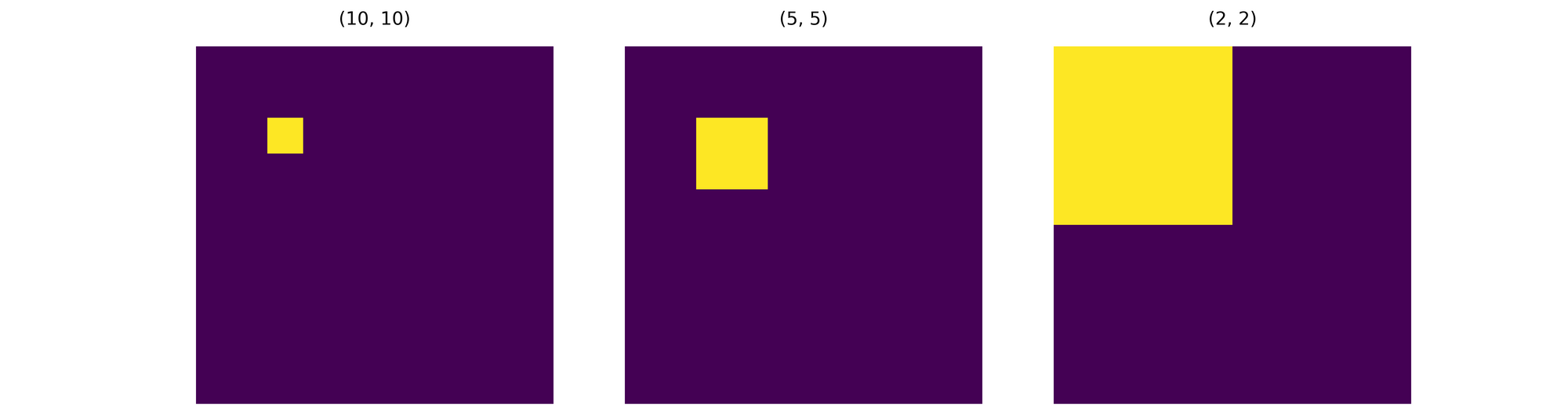
Picture 2
Now allow us to try and recreate the second picture on the proper the place the yellow pixel is positioned within the backside proper nook. In the identical vane, when the picture is max-pooled twice utilizing a (2, 2) kernel then the yellow pixel will now be positioned at index [1, 1] as max pooling brings essentially the most salient function of the picture into focus.
image_2 = np.zeros((10, 10))
image_2[-3, -3] = 1.0Once more, utilizing the capabilities supplied we will see that the ensuing picture bares a resemblance to the hand drawn illustration.
visualize_pooling(image_2, 2, dpi=200)
Evaluating Pictures
Wanting on the two reference photos, the yellow pixels had been initially 5 rows and 5 columns of pixels aside. Nevertheless, after the primary max-pooling course of, the pixels turned simply two rows and two columns of pixels aside till they turned only one row and one column aside by the second iteration of max-pooling. And naturally, if max-pooling had been to be carried out another time, solely the yellow pixels might be returned in each cases.
That is basically what translation invariance entails. Pooling make it such that no matter the place the article of curiosity could be moved to on the picture, on the finish of the day, it is options might be positioned in roughly the identical place when max-pooled sufficient occasions.
Equivariance and Invariance Working in Tandem
On this part we might be looking at how translation equivariance and translation invariance work in tandem. In an effort to do that we are going to once more be utilizing the picture within the subsequent part as a reference picture.
Reference Picture

Utilizing the reference picture, we first must detect edges within the picture utilizing the Sobel vertical edge detection filter beforehand outlined. When that is carried out we then move the detected edges as parameter to the pooling visualization operate and undergo 6 iterations of max pooling. The result’s displayed beneath with the important edges of the picture being constrained right into a 6 x 9 pixel picture by the sixth iteration.
#  detecting edges in picture
edges = convolve('picture.jpg', filter=sobel_y)

#  going by way of 6 iterations of max pooling
visualize_pooling(np.array(edges), 6, dpi=500)Mirrored Picture

#  detecting edges in picture
edges_2 = convolve('image_2.jpg', filter=sobel_y)

#  going by way of 6 iterations of max pooling
visualize_pooling(np.array(edges_2), 6, dpi=500)
Now utilizing the mirrored model of the reference picture and repeating the steps as outlined within the earlier part produces the illustration that follows. From mentioned illustration, we will see translation equivariance in motion by advantage of the truth that the identical actual options have been extracted although the place of the article of curiosity has modified. Additionally, we will see translation invariance in motion by lieu of the truth that though options are positioned in numerous positions, they’re progressively introduced towards the identical place till they’re in roughly the identical location in a 6 x 9 pixel body.
Comparability Picture

Even when coping with two fully totally different photos, one can nonetheless see translation invariance in motion. Take into account the picture above, when in comparison with the reference picture, the article of curiosity on this picture is positioned on the other facet. Nevertheless by the sixth epoch, it is most vital options are additionally now positioned in the identical approximate location as these of the reference picture.
#  detecting edges in picture
edges_3 = convolve('image_3.jpg', filter=sobel_y)

#  going by way of 6 iterations of max pooling
visualize_pooling(np.array(edges_3), 6, dpi=500)On this article. we have now been in a position to have a look at two of the options of convolutional neural networks which make them fairly strong. It is fairly fascinating that these two options haven’t truly been purposefully programed into the neural community relatively they’re bye merchandise of processes that make a CNN what it it.